TECHNICAL PAPER

 

Use of Rayleigh and Love waves in seismic surface wave testing

 

 

M S Islam; G Heymann

Correspondence

 

 

---

ABSTRACT

Seismic surface wave tests are widely used in geotechnicai engineering due to their noninvasive and cost-effective approach in obtaining important soil parameters such as the small strain shear modulus (G₀) by measuring shear wave velocity (Vs). While conventional tests focus on measuring Rayleigh waves due to their easy generation and detection in the field, Love waves are often overlooked due to challenges in generating and detecting them. This study investigated the utilisation of both Rayleigh and Love waves to obtain shear wave velocity profiles using experimental and synthetic data. Two methods were explored for generating Love waves - using a horizontal harmonic source, and also employing a horizontal impact source. Signal processing code was developed to analyse the surface wave signals and to calculate dispersion data. By conducting discrete and joint inversions with the experimental and synthetic dispersion data, the variation in the shear wave velocity profiles was evaluated. The findings demonstrated that employing both Rayleigh and Love waves in joint inversion reduced the variation in the shear wave velocity profile compared to using Rayleigh waves alone, but only when Love wave signals with low noise levels were available.

Keywords: seismic surface wave test, Rayleigh waves, Love waves, joint inversion, CSW, SASW

---

 

 

INTRODUCTION

Seismic testing methods are important in geotechnicai engineering for characterising shallow subsurface stratigraphy and stiffness, primarily by measuring the shear wave velocity (Vs) profile, which allows quantification of soil parameters such as the small strain shear modulus (G₀) (Ganji et al 1998). In a continuum, seismic energy is mainly propagated by two types of waves - body waves (compression and shear waves) and surface waves (Rayleigh and Love waves). Surface waves are generated near the surface when seismic energy propagates through mediums bounded by a free surface. Rayleigh waves have particle motion in the vertical plane in the direction of propagation with a retrograde elliptical orbit. Love waves have particle motion perpendicular to the direction of propagation in planes parallel to the ground surface (Strobbia 2003).

Surface wave analysis aims to determine the Vs profile by solving the inverse problem using experimental dispersion data. This requires acquisition of surface wave data and processing signals to generate experimental dispersion data, and optimising model parameters during inversion analysis. However, the inversion problem is non-unique, which can pose challenges in obtaining reliable solutions from experimental data (Foti et al 2018).

Most surface wave tests, such as Continuous Surface Wave (CSW) (Menzies & Matthews 1996), Spectral Analysis of Surface Waves (SASW) (Stokoe et al 2004), and Multi-Channel Analysis of Surface Waves (MASW) (Park et al 1999), rely on Rayleigh wave velocity (Vr) to obtain the shear wave velocity profile. This is due to the ease of generating and detecting Rayleigh waves compared to Love waves. Love waves, which require specific generating conditions, have received less attention in seismic surface wave testing, making their application relatively new in geotechnical site investigations.

This paper explores the effects of joint inversions using both active Rayleigh waves and Love waves measured using both harmonic and impact sources to estimate the shear wave velocity profile. This was compared with discrete inversions that rely solely on Rayleigh waves. CSW and SASW testing methods were implemented at two test sites, and synthetic dispersion data was also considered to further assess the performance of discrete and joint inversions.

 

BACKGROUND

Love waves

Love waves induce particle motion perpendicular to the direction of propagation in planes parallel to the ground surface. These waves are only present in layered bodies (heterogeneous mediums) where a surface waveguide exists, consisting of a surface layer above a substrate layer (Figure 1). To generate Love waves, the surface layer must fulfil the condition:

 

 

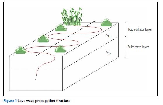
Vs₁ < Vs₂

Where: Vs₁ and Vs₂ are defined as the shear wave phase velocities in the surface layer and substrate, respectively. Love waves can be generated in normally dispersive ground profiles but not in uniform or inversely dispersive profiles.

Similar to Rayleigh waves, Love waves are dispersive, with their phase velocities depending on the frequency and exhibiting multimodal behaviour. However, they are less susceptible to higher mode generations compared to Rayleigh waves (Martin et al 2014; Safani et al 2005). Despite these advantages, the use of Love waves for seismic surface wave testing has been less popular due to challenges in generating strong Love waves and the fact that Love wave measurements require horizontal geophones.

To generate Love waves, various sources have been used, such as the horizontal traction shear beam (Foti et al 2018), hammer impact (Haines 2007), and harmonic sources such as horizontal vibroseis. Inverting Love wave dispersion data follows similar principles to Rayleigh wave data inversion, but the forward solution for Love waves requires only the shear wave velocity, as they are independent of compressional wave velocity.

Though some researchers have investigated site characterisation using Love waves, certain fundamental questions, such as near field effects and limitations due to source frequency, remain underexplored (Foti et al 2018).

Continuous Surface Wave (CSW) test

The conventional CSW test utilises frequency-controlled vibrators to generate steady-state Rayleigh waves along the ground, while an array of vertical geo-phones detects the surface wave motion (Menzies & Matthews 1996). The vibrator is stepped through a set of frequencies to generate a range of wavelengths. Electromagnetic vibrators, controlled by a signal generator and power amplifier, as well as mechanical vibrators driven by an electrical motor and controlled by a variable frequency drive, have been employed (Heymann 2013). Both types of vibrators can also generate transient signals that sweep through a range of frequencies within a specified time.

Spectral Analysis of Surface

Waves (SASW) test

This test uses an impact source accompanied by a pair of receivers (two or three) placed at known distances from the source, with the receivers spaced at a distance (∆X) equal to the source offset. To generate the desired frequency ranges, sledgehammers and drop weights of varying masses are utilised (Stokoe et al 2004).

During the Spectral Analysis of Surface Waves (SASW) tests, it is essential to consider the signal-to-noise ratio (SNR) of the impact source's signal, as the energy of the signals deteriorates with distance. To enhance the SNR, SASW employs geometrical array configurations and stacking (repeated shots).

 

EXPERIMENTAL WORK

CSW and SASW Love wave sources

The CSW Love wave tests were carried out using both steady-state signals and transient (sweep) signals. For the steady-state Rayleigh wave Continuous Surface Wave (CSW) tests, high-frequency and low-frequency mechanical vibrators were used. The high-frequency vibrator had a total eccentric mass of 1.06 kg, an eccentricity of 23.6 mm, and operated at frequencies up to 90 Hz. The low-frequency vibrator had a total eccentric mass of 11.1 kg, an eccentricity of 31.8 mm, and operated at frequencies up to 22 Hz. The Variable Frequency Drive (VFD) converted the AC supply into the desired operating frequency for the vibrators.

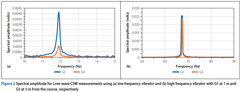
The evaluation of vibrator performance was conducted by plotting the spectral amplitudes of the geophone signals (Figure 2). The results indicate that the peak frequencies obtained from both geophone 1 (closest to the source) and geophone 5 (farthest from the source) were similar. By analysing the spectral amplitude plots, the frequency required for calculating the Love wave velocity, V_L, was determined.

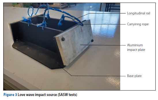
For Love wave SASW testing, a specially designed steel impact source was used, inspired by Haines' shear wave seismic source (Haines 2007). The impact source featured 12 mm thick mild steel plates with two inclined impact plates and two longitudinal rails welded to a base plate holding shear spikes for shear coupling. Two lengths of shear spikes were employed based on ground conditions, with shorter spikes for firm ground and longer spikes for soft ground. Each impact plate had a 10 mm aluminium plate bolted to provide sacrificial protection and reduce noise during striking as shown in Figure 3.

 

 

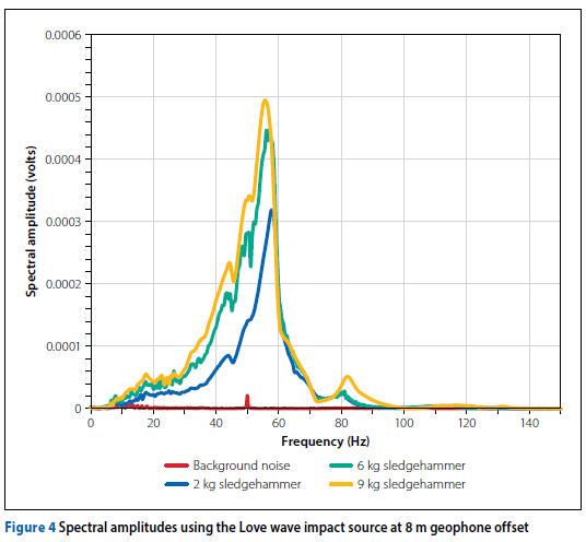
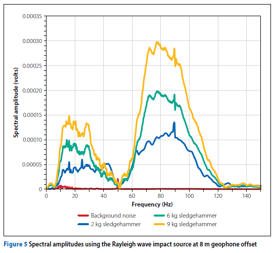
For the SASW test three sledgehammers (respectively with a mass of 2 kg, 6 kg and 9 kg) were used as impact source. To assess the signal-to-noise ratio (SNR), measurements of the background noise were conducted and compared to the spectral amplitude produced by the sledgehammers. Figure 4 illustrates the comparison of spectral amplitudes between the background noise and the individual sledgehammer signals for the Love wave steel impact source. For comparison, the spectral amplitude of the Rayleigh wave is depicted in Figure 5.

 

 

 

 

Test sites

CSW and SASW tests were performed at two sites, namely the University of Pretoria Hillcrest Campus in Pretoria, South Africa, and a bentonite mine near the town of Vredefort in the Free State Province, known as the Wind Africa site. The geology at both sites was determined from available test pit and borehole results.

At the University of Pretoria site, the subsurface consisted of residual andesite (lava) of the Hekpoort formation, Pretoria Group. The test pit profiles showed an increase in stiffness with depth due to reduced weathering down to the bedrock at approximately 3 m. No perched water tables or seepage zones were encountered during the test pit excavations, and the selected seismic test site had a reasonably flat topography with grass and thick scrub vegetation on either side of the test area.

At the Wind Africa test site the test pit profiles consisted of black, stiff silty clay near the surface, transitioning to olive-brown sandy clay at greater depths, both classified as high-plasticity clay (CH) and high-plasticity silt (MH), respectively. No water table was encountered during the test pit excavations, and drilling revealed hard to very hard norite or anorthosite bedrock at approximately 12 m below the surface (Da Silva et al 2019). Standard penetration tests (SPT) data showed an increase in stiffness with depth, with SPT N values increasing from about 17 at 1 m to refusal at 15 m. The chosen test area had a flat terrain with vegetation comprising mainly grass.

Experimental setup

CSW tests

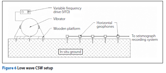
For the Love wave tests, the same vibrators were utilised as for the Rayleigh wave Continuous Surface Wave (CSW) tests, but they were placed horizontally and securely fastened to a wooden base (1.22 m X 0.55 m) with steel screw plates for shear coupling with the ground surface. The vibrator was oriented perpendicularly to the horizontal geophone array as shown in Figure 6. The ground detection system consisted of five geophones with a resonant frequency of 4.5 Hz for both vertical and horizontal geophones. A 24-channel seismograph recorded the output from the geophones.

 

 

SASW tests

The SASW tests utilised three sledgehammers (respectively with a mass of 2 kg, 6 kg and 9 kg) to produce seismic energy across different frequencies. The mass of the impact source influenced the generated energy content, resulting in varying frequency ranges for the distributed energy. A trigger switch on each sledgehammer facilitated the acquisition process upon impact.

For Rayleigh wave SASW tests, the sledgehammers were struck against a 20 mm thick metal base plate (170 mm diameter) buried 50 mm into the ground to enhance signal quality.

In the SASW test layout, two geophones were used, and the distances between the source and the nearest geophone ranged from 1 m to 16 m. The common receiver midpoint configuration was applied, involving the relocation of both the source and receivers to a fixed centre line. To assess lateral variations in the soil medium, two shots (forward and reverse shots) were conducted during the test. Each shot consisted of four strikes to enable data stacking and reduce the impact of background noise.

Test specifications

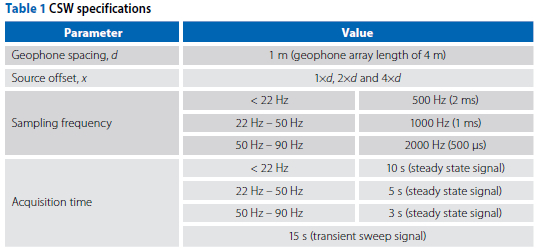
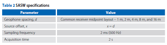
Tables 1 and 2 present the different experimental arrangements that were used for the CSW and SASW tests.

 

 

 

 

Data inversion

The experimental dispersion data was used to estimate the one-dimensional shear wave velocity profile of the chosen sites. This was achieved through the software, Dinver (3.3.6), which implemented a neighbourhood optimisation algorithm (Wathelet 2008). For this study two inversion scenarios were considered. Firstly, a discrete Rayleigh wave inversion was conducted using only Rayleigh wave dispersion data, and secondly a joint inversion was conducted using both Rayleigh and Love wave dispersion data. A weighting of 1.0 was used for all dispersion data points in the Dinver inversion analysis to ensure an unbiased comparison of the discrete and joint inversion strategies.

Upon conclusion of each inversion analysis, Dinver (3.3.6) provided the minimum misfit value (M_m) computed for each optimisation run. The misfit value provided a numerical indicator of the fit between the experimental and theoretical dispersion curves. The misfit value (M_f) was defined as:

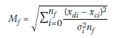
Where:

X_di = velocity of the experimental curve at frequency f_i

x_ci = velocity of the calculated theoretical curve at frequency f_i

σ_i = standard deviation of the frequency samples

n_f = number of frequency samples considered.

The profiles with a misfit within 10% of the minimum misfit were used to evaluate the uncertainty in the Vs profiles for each inversion approach. No sensitivity analysis tests were conducted with regard to parameterisations.

Data processing

CSW

The signal processing of the CSW results was done using Python signal processing code developed during the project and which is available in Islam (2022). The signal data was recorded in the time domain and a Fast Fourier Transformation (FFT) was conducted to convert it to the frequency domain. The maximum value of the frequency response spectrum was used to determine the dominant frequency of the seismic waves. At this frequency the phase angles at each geophone were calculated using Equation 1, and if required it was unwrapped to produce a phase angle-distance plot.

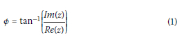
Where:

φ = phase angle (rad)

z = frequency vector at dominant frequency.

A linear regression analysis was conducted on the phase angle against geophone distance to determine the line of best fit together with the coefficient of determination (R²) to evaluate the fit. The slope of the best fit linear line was used to calculate the phase velocity for each frequency using Equation 2. These phase velocities were used to plot the respective dispersion data points at each frequency.

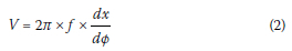
Where:

V = velocity (m/s)

f = vibrator frequency (Hz)

= inverse of slope of phase angle distance regression line.

SASW

Python signal processing code was also developed to analyse the SASW test data and is available in Islam (2022). The signal processing included analysis of the spectral amplitude, coherence, and phase difference. Domain transformation from time to frequency was again done, which allowed the spectral amplitude to be calculated for each geophone. The wrapped phase difference was calculated using the cross-power spectrum of the two geophones. Equations 3 to 5 were used to calculate the respective functions.

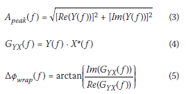
Where:

Y(f) = Fourier transformation at geophone 1

X*(f) = complex conjugation of Fourier transformation at geophone 2

G_Yx(f) = cross-power spectrum

A_peak = peak or spectral amplitude (volt)

Δφ_wrap(f) = wrapped phase difference (rad).

Acceptable data was selected through the evaluation of the spectral amplitude plot, the wrapped phase difference plot, and the coherence function. The selection process is commonly referred to as 'masking' of the data. A coherence criterion (γ² > 0.9) was applied to the results to identify frequency regions with high signal quality (Nazarian & Stokoe 1986). Upon unwrapping the phase difference, the phase velocity at each respective frequency was calculated using Equation 6, and dispersion curves were constructed. A final composite dispersion curve was assembled by merging each of the individual dispersion curves measured for each test configuration.

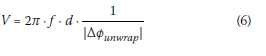
Where:

V = phase velocity (m/s)

f = frequency (Hz)

d = geophone spacing (m)

Δφ_unwrap = unwrapped phase difference (rads).

 

RESULTS AND DISCUSSION

Synthetic dispersion data

A theoretical approach using synthetic Rayleigh and Love wave dispersion data was used to compare the discrete and joint inversion approaches. A theoretical model with two layers and a half-space layer, with properties as shown in Figure 7, was used to generate synthetic dispersion data. The forward calculation for the Rayleigh and Love models was calculated using the formulation of Wathelet (2005) and is available as the gpdc package, which is part of the Geopsy software suite of open-source software for geophysical research. The forward calculation formulation is based on the eigenvalue problem described by Thomson (1950) and Haskell (1953), subsequently modified by Knopoff (1964), Dunkin (1965) and Herrmann (1994). The values of the shear wave velocity (Vs) and compression wave velocity (Vp) were chosen to give a normally dispersive profile with a Poisson's ratio close to 0.25, which is typical for soils above the water table. Karray and Lefebvre (2008) have shown that the choice of Poisson's ratio affects both the calculation of synthetic data and inversion analysis of dispersion data, and hence, for consistency, a constant Poisson's ratio was used to calculate the synthetic dispersion data. Random noise was superimposed on some of the synthetic dispersion data to investigate the effect of the quality of the dispersion data on the performance of the inversion strategies.

 

 

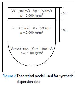
The following inversion cases were analysed:

A. Discrete inversion - Rayleigh waves (0% noise)

B. Joint inversion - Rayleigh waves (0% noise) and Love waves (0% noise)

C. Joint inversion - Rayleigh waves (0% noise) and Love waves (10% noise)

D. Joint inversion - Rayleigh waves (10% noise) and Love waves (0% noise)

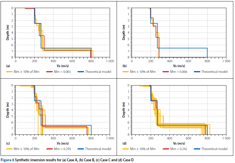
An inversion analysis was conducted on the synthetic dispersion data to find theoretical Vs profiles with dispersion curves that best match the dispersion data. The estimated Vs profiles were evaluated using the minimum misfit value (M_m) and Vs profiles with a misfit (M_f) within 10% of the minimum misfit (M_m). Figure 8 shows the results. The blue Vs profile is the theoretical model shown in Figure 7 which was used to generate synthetic dispersion data. This Vs profile can be used as a reference to judge how successful the inversion analysis was in recovering the original theoretical ground model. The red Vs profile is the profile with the minimum misfit and the yellow profiles are Vs profiles with a misfit within 10% of the minimum misfit.

It was noticed that the number of Vs profiles approximated by Case A (Figure 8a) and Case B (Figure 8b) were significantly less than for Case C (Figure 8c) and Case D (Figure 8d) when noise was added. The reason is that the minimum misfit values for Cases A and B were small, and therefore 10% of M_m was a small range and few of the recovered profiles had misfit values within this range. Both inversion Cases A and B provided similar recoveries of the original Vs profile with reasonable estimates of the Vs profiles within the misfit limits. However, it is interesting that in some cases the joint inversion (Case B) did not recover the stiff layer below 6.5 m. Upon the addition of noise, the number of approximated Vs profiles increased (Cases C and D) and a greater variation was observed between the upper-bound and lower-bound Vs profiles. It is interesting to note that the minimum misfit value is more sensitive for the addition of noise than whether a discrete of joint inversion analysis was conducted. For Cases A and B, without noise, the minimum misfit values were 0.065 and 0.066 respectively, and for Cases C and D, where noise was added, the misfit values were about four times higher at 0.293 and 0.242.

The estimated Vs profiles were also evaluated in terms of their variation at different depths. The Vs variation was taken as the difference between the highest and lowest Vs value at a particular depth of all profiles with a misfit within 10% of the minimum misfit. The variation in the Vs was used as an additional indicator to assess the performance of the different inversion strategies. This is a useful indicator, because when field data is used, no theoretical profile exists against which the performance of an inversion strategy can be compared. A large variation in Vs indicates that the certainty with which the Vs profile can be recovered during the inversion process is poor. The difference between the maximum and minimum estimated Vs profiles was determined up to a depth of 7 m.

From Figure 9 it was seen that between depths of 1 m and 5 m (the top two layers), the variation in the Vs was below 140 m/s for all four inversion cases. Layers with a thickness of less than 1 m were ignored as this was less than the layer thickness that could be resolved based on the minimum wavelength measured by the theoretical dispersion points.

 

 

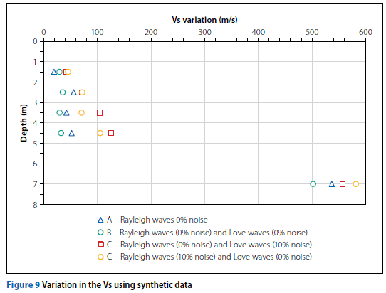
Figure 9 shows that, in general, a joint inversion incorporating good quality Rayleigh and Love wave dispersion data (Case B) produced a smaller Vs variation than a discrete inversion analysis using only Rayleigh wave data (Case A). This was observed for four out of the five cases. Upon the addition of noise, the quality of the inversion results deteriorated. For all depths the Vs variation was greater for both Case C and Case D (10% noise for either Rayleigh or Love wave data) than that obtained from Case A and Case B (0% noise). Thus, the quality of the dispersion data significantly affected the inversion process and reduced the ability to accurately estimate the theoretical Vs profile.

University of Pretoria (UP) test site

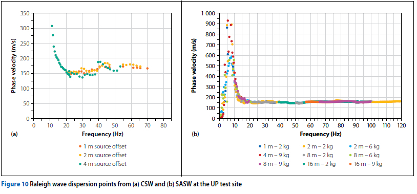
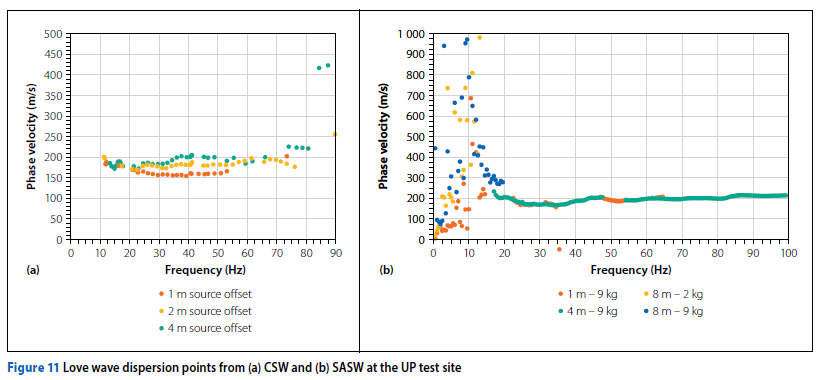
Each seismic test (CSW and SASW) was used to generate two experimental dispersion plots, one each for Rayleigh waves and Love waves, as shown in Figure 10 and Figure 11. It shows that higher modes of vibration existed for all four tests. A multimode analysis was not conducted as it would introduce additional uncertainties with regard to identifying the mode number or the possibility of superposed modes. Thus, for all the inversion analyses, only fundamental mode data was used. For the CSW Rayleigh waves, dispersion data between 10 Hz and 40 Hz were used, and dispersion data between 10 Hz and 35 Hz were used for the CSW Love waves. The fundamental mode for the SASW Rayleigh waves was between 10 Hz and 100 Hz, and between 10 Hz and 40 Hz for the SASW Love waves. SASW data below 10 Hz was ignored as this was beyond the limit of the energy that the impact sources could produce, as shown in the large scatter of the data points below 10 Hz.

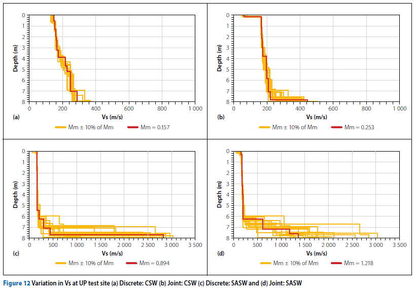
Inversion analyses were performed to find the variation in the Vs profiles by considering the upper-bound and lower-bound Vs profiles within the limits of Mm ±10% of Mm. The smaller the variation in the Vs, the better the Vs profile could be approximated. Figure 12 illustrates the variation in the Vs when using discrete and joint inversions for CSW and SASW approaches, respectively. By limiting the frequency ranges of the dispersion points, the minimum depth that could be resolved was 2 m.

As shown in Figure 12b, between 2 m and 6 m, the joint inversion for the CSW approach produced a smaller variation in the Vs than that from the discrete inversion Figure 12a. For depths greater than 7 m, it was observed that the discrete inversion produced a smaller variation in Vs compared to the joint inversion. With regard to the SASW test, it was observed from Figure 12c that the discrete inversion produced a smaller variation in the Vs than the joint inversion for depths between 2 m and 4 m, and for depths between 5 m and 6 m the joint inversion produced a smaller Vs variation than the discrete inversion. For depths greater than 6 m, both discrete and joint inversions produced similar variations in the Vs. Based on Figure 12, the CSW joint inversion appears to improve the results, whereas the SASW joint inversion does not.

Wind Africa test site

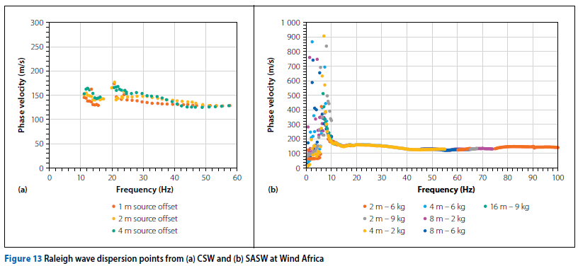
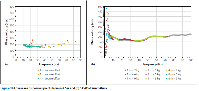
CSW and SASW tests were used to generate Rayleigh wave and Love wave dispersion data, which was then used for the inversion analysis (Figure 13 and Figure 14). Once again it was noticed that higher modes of vibration existed for all four tests. Multimode analysis was not conducted to avoid additional uncertainties, as had been explained above. Dispersion data between 10 Hz and 60 Hz was considered for the CSW Rayleigh wave, and dispersion data between 10 Hz and 40 Hz was considered for the CSW Love waves. On the other hand, SASW Rayleigh waves between 10 Hz and 100 Hz and SASW Love waves between 10 Hz and 40 Hz were considered during the inversion process. SASW data below 10 Hz was ignored due to the limit in the energy that the impact sources could produce.

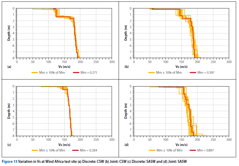
The variation in the Vs was again calculated by considering the upper-bound and lower-bound Vs profiles within the limits of Mm ±10% of Mm. The variations in the Vs for the discrete and joint inversions using CSW and SASW tests respectively are shown in Figure 15.

Figure 15 shows that the discrete inversion provided a smaller variation in the Vs profiles when compared to the Vs profiles obtained from the joint inversion variation. This was observed for both the CSW and SASW tests.

 

CONCLUSION AND RECOMMENDATIONS

In this study the focus was on investigating the effect of utilising both Love waves and Rayleigh waves to determine the shear wave velocity (Vs) of the ground. Signal processing code was written to calculate dispersion data for both CSW and SASW tests. Love waves were successfully generated using a vibratory source for CSW tests and an impact source for SASW tests, and their signals were easily detected by horizontal geophones, allowing similar processing to that of Rayleigh wave tests.

For both test sites, higher modes of vibration were observed for both Rayleigh and Love waves, with Love waves having less tendency of generating higher modes compared to Rayleigh waves. This observation agrees with the findings of Safani et al (2005) and Martin et al (2014).

Joint inversions using Rayleigh and Love waves were performed to estimate the Vs profiles using synthetic and experimental dispersion data. With synthetic data, joint inversion resulted in less variation in the Vs profiles compared to discrete inversion,

provided the data contained no noise. However, when 10% noise was introduced to the dispersion data, joint inversion led to a higher variation in the Vs profiles compared to using only Rayleigh wave data without noise. For the inversion analysis of experimental data at the two test sites, joint inversion produced a larger variation in the Vs profiles compared to discrete inversion using Rayleigh wave data only. These findings indicate that joint inversion of Rayleigh and Love waves improves the estimation of the Vs profile only when Love wave signals with low noise levels are available.

 

REFERENCES

Da Silva, T S, Haigh, S K, Elshafie, M Z E B, Jacobsz, S W, Day, P W & Osman, A S 2019. Preparations for field testing for the performance validation of piled wind turbine foundations in expansive clays. Proceedings, 17th African Regional Conference on Soil Mechanics and Geotechnical Engineering, 7-9 October, Cape Town.         [ Links ]

Dunkin, J W 1965. Computation of modal solutions in layered, elastic media at high frequencies. Bulletin of the Seismological Society of America, 55: 335-358.         [ Links ]

Foti, S, Hollender, F, Garofalo, F, Albarello, D, Asten, M, Bard, PY et al 2018. Guidelines for the good practice of surface wave analysis. A product of the InterPACIFIC project. Bulletin of Earthquake Engineering, 16(6): 2367-2420.         [ Links ]

Ganji, V, Gucunski, N & Nazarian, S 1998. Automated inversion procedure for spectral analysis of surface waves. Journal of Geotechnical and Geoenvironmental Engineering, 124(8): 757-770.         [ Links ]

Haines, S S 2007. A hammer-impact, aluminium, shear-wave seismic source. Technical Report OF 07-1406. Reston, VA: US Geological Survey.         [ Links ]

Haskell, N A 1953. The dispersion of surface waves on multilayered media. Bulletin of the Seismological Society of America, 43: 17-34.         [ Links ]

Herrmann, R B 1994. Computer Programs in Seismology, Vol IV. St Louis, MO: St Louis University.         [ Links ]

Heymann, G 2013. Vibratory sources for continuous surface wave testing. In Coutinho, R Q & Mayne, P W (Eds), Geotechnical and Geophysical Site Characterization 4, London: Routledge, pp 1381-1386.         [ Links ]

Islam M S 2022. Use of Rayleigh and Love waves in seismic surface wave testing. Master's Dissertation. University of Pretoria.         [ Links ]

Karray, M & Lefebvre, G 2008. Significance and evaluation of Poisson's ratio in Rayleigh wave testing. Canadian Geotechnical Journal, 45: 624-635.         [ Links ]

Knopoff, L 1964. A matrix method for elastic wave problems. Bulletin of the Seismological Society of America, 54: 431-438.         [ Links ]

Martin, A, Yong, A K & Salomone, L A 2014. Advantages of active Love wave techniques in geophysical characterizations of seismographic station-case studies in California and the central and eastern United States. Proceedings, 10th U.S. National Conference on Earthquake Engineering, 21-25 July, Anchorage, AK, p 11.         [ Links ]

Menzies, B & Matthews, M 1996. The continuous surface-wave system: A modern technique for site investigation. Special Lecture, Indian Geotechnical Conference, Madras, pp 11-14.         [ Links ]

Nazarian, S & Stokoe, K H 1986. Use of surface waves in pavement evaluation. Transportation Research Record, 1070: 132-144.         [ Links ]

Park, C B, Miller, R D & Xia, J 1999. Multichannel analysis of surface waves. Geophysics, 64(3): 800-808.         [ Links ]

Safani, J, O'Neill, A, Matsuoka, T & Sanada, Y 2005. Applications of Love wave dispersion for improved shear-wave velocity imaging. Environmental and Engineering Geophysics, 10(2): 135-150.         [ Links ]

Stokoe, K H, Joh, S-H & Woods, R D 2004. Some contributions of in situ geophysical measurements to solving geotechnical engineering problems. Proceedings, 2nd International Conference on Site Characterization, 19-22 September, Porto, Portugal, pp 97-132.         [ Links ]

Strobbia, C 2003. Surface wave methods. Acquisition, processing, and inversion. PhD Thesis. Turin, Italy: Politecnico di Torino.         [ Links ]

Thomson, W T 1950. Transmission of elastic waves through a stratified solid medium. Journal of Applied Physics, 21: 89-93.         [ Links ]

Wathelet, M 2005. Array recordings of ambient vibrations: Surface-wave inversion. PhD Thesis. Liège, Belgium: Université de Liège.         [ Links ]

Wathelet, M 2008. An improved neighborhood algorithm: Parameter conditions and dynamic scaling. Geophysical Research Letters, 35(9): 1-15.         [ Links ]

 

 

Correspondence:
M S Islam
PeraGage
Block C, Irene Link, Centurion, Pretoria 0157, South Africa
E: mohammed@peragage.com

G Heymann
Department of Civil Engineering, University of Pretoria
Private Bag X20, Hatfieid, Pretoria 0028, South Africa
E: gerhard.heymann@up.ac.za

 

 

 

MOHAMMED ISLAM (AMSAICE) is a Candidate Geotechnical Engineer with a strong academic foundation and subsequent professional experience. He graduated with distinction in Civil Engineering in 2018, followed by an Honours Degree in Geotechnical Engineering from the University of Pretoria, and in 2021 a Master's in Geotechnicai Engineering from the same university. Currently he works as a geotechnicai design engineer at PeraGage, where he specialises in the design and supervision of lateral support systems, excavations, piling systems, and slope stability assessments for both iocai and international ventures.

 

 

PROF GERHARD HEYMANN (Pr Eng, FSAICE), who is a professor in the Department of Civil Engineering at the University of Pretoria, holds BEng, BEng(Hons) and MEng degrees from the same university, and a PhD from the University of Surrey. He has been involved with teaching and research in geotechnical engineering for many years. His fields of interest include the characterisation of soil behaviour and its application in geotechnical engineering. He is a past chairman of the SAICE Geotechnical Division, and aiso a recipient of the Jennings Award for the best geotechnicai paper by a South African author. In addition he was awarded the South African Geotechnicai Medai in 2018 for his contribution to geotechnicai engineering in South Africa.