RESEARCH ARTICLE

 

Benign interpolation of noise in deep learning

 

 

Marthinus Wilhelmus Theunissen^{I, II}; Marelie H. Davel^{I, II}; Etienne Barnard^{I, II}

^IMultilingual Speech Technologies, North-West University, South Africa. Email: Marthinus Wilhelmus Theunissen tiantheunissen@gmail.com (corresponding), Marelie H. Davel marelie.davel@gmail.com, Etienne Barnard etienne.barnard@gmail.com
^IICentre for Artificial Intelligence Research, South Africa

 

 

---

ABSTRACT

The understanding of generalisation in machine learning is in a state of flux, in part due to the ability of deep learning models to interpolate noisy training data and still perform appropriately on out-of-sample data, thereby contradicting long-held intuitions about the bias-variance tradeoff in learning. We expand upon relevant existing work by discussing local attributes of neural network training within the context of a relatively simple framework. We describe how various types of noise can be compensated for within the proposed framework in order to allow the deep learning model to generalise in spite of interpolating spurious function descriptors. Empirically, we support our postulates with experiments involving overparameterised multilayer perceptrons and controlled training data noise. The main insights are that deep learning models are optimised for training data modularly, with different regions in the function space dedicated to fitting distinct types of sample information. Additionally, we show that models tend to fit uncorrupted samples first. Based on this finding, we propose a conjecture to explain an observed instance of the epoch-wise double-descent phenomenon. Our findings suggest that the notion of model capacity needs to be modified to consider the distributed way training data is fitted across sub-units.
CATEGORIES: • Computing methodologies ~ Machine learning • Computing methodologies ~ Neural networks • Theory of computation ~ Sample complexity and generalisation bounds

Keywords: deep learning, machine learning, learning theory, generalisation

---

 

 

1 INTRODUCTION

Advantages of deep learning models include their scalability to high-dimensional data, effective optimisation, and performance on data that was not optimised for (Goodfellow et al., 2016). The latter is arguably the most important benefit. Machine learning, as a whole, has seen much progress in recent years, and deep neural networks (DNNs) have become a cornerstone in numerous important domains such as computer vision, natural language processing and bioinformatics. Somewhat ironically, this application potential has resulted in the development of theoretically principled guidelines lagging behind implementation-specific progress.

A particular example of one such open theoretical question is how to reconcile the observed ability of over-paramerised DNNs to generalise, with classical notions of generalisation in machine learning.

A widely accepted principle with which to reason about generalisation in machine learning, is that generalisation ability is linked to the complexity of the hypothesis space, and that a model's representational capacity should be restricted so as to prevent it from approximating unrealistically complex functions (Vapnik, 1999). Such highly complex functions are not expected to be applicable to the task being performed, and are usually a result of overfitting the spurious correlations found in the finite sample of training examples. Many complexity metrics have been proposed and adapted in an attempt to consolidate this intuition, however, these metrics have failed to fully account for the generalisation observed in deep learning models in general circumstances (Kawaguchi et al., 2017; Shalev-Shwartz & Ben-David, 2014; Sun et al., 2015).

An influential paper by Zhang et al. (2017) demonstrated that: (1) DNNs can efficiently fit various types of noise and still generalise well, and (2) contemporary explicit regularisation is not required to enable good generalisation. These findings are in apparent contradiction with complexity-based principles of generalisation: deep learning models are shown to have representational capacity large enough to approximate extremely complex functions (potentially memorising the entire, possibly noisy, data set) and still have very low out-of-sample test error.

In this paper we further investigate the effect of noise in training data with regards to generalisation. Where Zhang et al. (2017) contributed towards the understanding of generalisation by pointing out misconceptions with regards to model capacity and regularisation, our contribution is to provide insight into a particular phenomenon that can (at least partially) account for the observed ability of a DNN to generalise in a very similar experimental framework. Specifically, we show that noise in the training data can be isolated from true task information by fitting sub-units of a network to feature information from samples that are locally similar. This simple characteristic prevents the sub-units fitted to noise from having an effect on predictions made on noiseless test data. The current work is an extension and refinement of that in Theunissen et al. (2019), extending Section 4 with additional results (as described in that section), and introducing an additional complementary investigation related to training with noise in Section 5, specifically addressing a phenomenon referred to as epoch-wise double descent.

We define noise as any input-output relationship that is not predictable, or not conducive to the model fitting the true training data or approximating the true data distribution. The following types of noise are investigated (detailed definitions are provided in Appendix B):

1. Label corruption: The training label of an affected sample is replaced with an alternative selected uniformly from all other possibilities.

2. Gaussian input corruption: All the input features of an affected sample are replaced with Gaussian noise with a mean and standard deviation equal to that of the uncorrupted sample.

3. Structured input corruption: For every affected sample, its input features are replaced by an alternative sample that is completely distinguishable from the true input but consistent per class. (For example, replacing selected images from one class with images of a completely different object from a different data set, but keeping the original class label.)

These types of noise were chosen to encompass those investigated in Zhang et al. (2017), place more emphasis on varying the noise, and still maintain the analytically convenient per-sample implementation of the analysis framework. It is possible to introduce other types of noise, such as stochastic corruptions in the feature representations at each layer within the architecture, or directly impeding the optimisation of the model. However, such noise is primarily useful in the study of regularisation techniques (dropout, weight decay, node pruning etc.) and not aligned with the goals of this paper, namely, to shed light on how a DNN with few or no regularising factors manages noisy data.

The empirical investigation is limited to extremely overparameterised multilayer perceptron (MLP) architectures with ReLU activations, and three related classification data sets. These architectures are simple enough to allow for efficient analysis but function using the same principles as more complex architectures. The three classification tasks are MNIST (LeCun et al., 1998), FMNIST (Xiao et al., 2017), and KMNIST (Clanuwat et al., 2018). These data sets are on the low end of the spectrum with regard to task difficulty, with FMNIST and KMNIST slightly more difficult than MNIST; both MNIST and FMNIST are widely used to investigate the theoretical properties of DNNs (Jastrzebski et al., 2019; Kawaguchi et al., 2017; Novak et al., 2018).

The following section (Section 2) discusses some notable related work that all have the goal of characterising generalisation in deep learning. In Section 3 we provide a theoretical perspective on DNN training that is useful to interpret the results that follow. The ability of an MLP to respond to noisy data is analysed and discussed in Section 4. Section 5 extends these results to address a specific phenomenon observed during training, namely epoch-wise double descent. Findings are summarised in the final section with a focus on implications relating to generalisation.

 

2 RELATED WORK

In the wake of the somewhat paradoxical results demonstrated in Zhang et al. (2017), much work has followed investigating the role of memorisation and generalisation in DNN learning (Arpit et al., 2017; Krueger et al., 2017; Neyshabur et al., 2017). Some of these investigations focus on the stability with which a model accurately predicts output values in the presence of varying input values. One popular approach is to analyse the geometry of the loss landscape at the optimum (Chaudhari et al., 2017; Hochreiter & Schmidhuber, 1997; Keskar et al., 2017).

This amounts to investigating the overall loss value within a region of parameter space close to the (near-)optimal parameterisation obtained by the training process. The intuition is that a sharper minimum or high curvature at the solution point indicates that the model will be sensitive to small perturbations in the input space. Logically, this will lead to poor generalisation. A practical problem with this approach is that it suffers heavily from the curse of dimensionality. This means that it is difficult to obtain an unbiased and consistent perspective on the error surface in high dimensional parameter spaces, which is the case in virtually all practical DNNs. The error surface is typically mapped with dimensionality reductions, random searches, or heuristic searches (Li et al., 2018). A conceptual problem is that the loss value is easily manipulated by weight scaling. For example, Dinh et al. (2017) showed that a minimum can be made arbitrarily sharp or flat with no effect on generalisation, by exploiting simple symmetries in the weight scales of networks with rectified units.

Another effort at imposing stability in model predictions is to enforce sparsity in the para-meterisation. The hope is that with a sparsely connected set of trainable parameters, a reduced number of input parameters will affect the prediction accuracy. Like complexity metrics, this idea is borrowed from statistical learning theory (Maurer & Pontil, 2012) and with regards to deep learning, it has seen more success in terms of improving the computational cost (Gale et al., 2019; Loroch et al., 2018) and interpretability of DNNs than in improving generalisation.

From a representational point of view, some have argued that overparameterised DNNs approximate functions that are inherently insensitive to input perturbations at the optima to which they converge (Montufar et al., 2014; Neal et al., 2018; Novak et al., 2018; Raghu et al., 2017; Rahaman et al., 2019). These investigations place a large emphasis on the design choices (depth, width, activation functions, etc.) and are typically exploratory by nature.

A promising approach proposed in Elsayed et al. (2018) and Jiang et al. (2019) investigates DNN generalisation by means of "margin distributions", a measure of how far samples tend to be from the decision boundary. These types of metrics have been successfully used to indicate generalisation ability in linear models such as support vector machines (SVMs); however, determining the decision boundary in a DNN is not as simple. Therefore, Jiang et al. (2019) used the first-order Taylor approximation of the distance to the decision boundary between the ground truth class and the second highest ranking class. They were able to use a linear model, trained on the margin distributions of numerous DNNs, to predict the generalisation error of several out-of-sample DNNs. This suggests that DNN generalisation is strongly linked to the type of representation the network uses to represent sample information throughout its layers.

Recent work has focused attention on the contribution of sub-units towards the network's overall generalisation ability, whether these were significantly smaller networks (Frankle & Carbin, 2019), or individual nodes (Davel et al., 2020). In Davel et al. (2020), specifically, several types of per-layer classifiers were constructed from the individual nodes of trained MLPs. These classifiers were shown to perform at levels comparable to the global network from which they were created. In effect, each node was shown to create a locally aware unit, that collaborated in order to solve the overall classification task. This is a perspective we build on in the remainder of this paper.

 

3 HIDDEN LAYERS AS GENERAL FEATURE SPACE CONVERTERS

It is useful for the analysis of Sections 4 and 5 to consider each hidden layer in an MLP as producing a learned representation, converting the feature space from one representation to another. At the same time, individual nodes act as local decision makers and respond to very specific subsets of the input space, as discussed below.

3.1 Per-layer feature representations

In a typical MLP, several hidden layers are stacked in series. The output layer is the only one which is directly used to perform the global classification task. The role that the hidden layers perform is one of enabling the approximation of the necessary non-linear function through the use of the non-linearities produced by their activation functions. In this sense, all hidden layers can be thought of as general feature space converters, where the behaviour of one dimension in one feature space is determined by a weighted contribution of selected dimensions in the preceding feature space, as illustrated in Figure 1.

3.2 Per-node decision making

Whereas every hidden layer produces a feature space, every node determines a single dimension in this feature space. Some insights can be gained by theoretically describing the behaviour of a node in terms of activation patterns in the preceding layer. Let a_lbe an activation vector at a layer l as a response to an input sample x. If Wl is the weight matrix connecting l and the previous layer I - 1 then:

where f_ais some element-wise non-linear activation function. For every node i in l the activation value is then:

where wⁱ_lis the row in matrix Wl connecting layer l - 1 and node i. This can be rewritten as

with 0 specifying the angle between the weight vector and the activation vector.

The pre-activation node value is determined by the cosine similarity of the two vectors, scaled by the product of the norm of the activation vector (in the previous layer) and the norm of the relevant weight vector (in the current layer). As a result, if the activation function is a rectified linear unit (ReLU) (Glorot et al., 2011) and a bias is not used, the angle between the activation vector and the weight vector has to be e (-90°, 90°) for the sample information to be propagated by the node. In other words, the node is activated for samples that produce an activation pattern in the preceding layer with a cosine similarity larger than 0 in terms of the weight vector. This criterion holds regardless of the activation or weight strengths. (When a bias is used, the threshold angles are different, but the concept remains the same.)

3.3 Samplesets

When training a ReLU-activated network, the corresponding weight vector is only updated to optimise the global error in terms of those specific samples for which a node is active, referred to as the "sample set" of that node (Davel, 2019). This is because weights are updated according to the gradients which can only propagate back through the network to the weight vector if the corresponding node is active. In this sense, the node weight vector acts as a dividing hyperplane in the feature space of the preceding layer. This hyperplane corresponds to the points where the weight vector is equal to zero (or the bias value if one is present). Samples which are located on one side of the hyperplane are prevented from having an effect on the weight vector values, and samples on the other side are used to update the weights, thereby dictating the behaviour of one dimension in the following feature space. The actual weight updates are affected by the representations of sample information in all the layers following the current one.

3.4 Summary

To summarise this perspective on ReLU-activated MLP training:

1. Hidden layers represent sample information in a feature space unique to every layer.

2. The representations of sample information are created on a per-dimension basis by the in-fan weight vector at each node, selecting and weighing the dimensions made available in the preceding layer.

3. A node is only active for samples with a directional similarity in the previous feature space.

4. These sets of samples (and only these) are used to update each in-fan weight vector during training and, by extension, the representation used by the following feature space.

5. The constitution of these sample sets are therefor a key component during training, and we expect that the characteristics of these sets can shed led on the training process, and generalisation ability of DNNs.

 

4 FITTING TRAINING NOISE

We now present our empirical exploration of DNN learning, using the context described above. The current work is an extension and refinement of that in (Theunissen et al., 2019), yielding more robust results through additional optimisation, more random initialisations, and one additional data set at a higher resolution (data corruption is varied over more increments). Consequently, we obtain a more detailed depiction of the changes in per-layer sample information representations. Unless stated otherwise, all results are averaged over at least 3 random initialisations and all error margins refer to the standard error.

4.1 Model performance

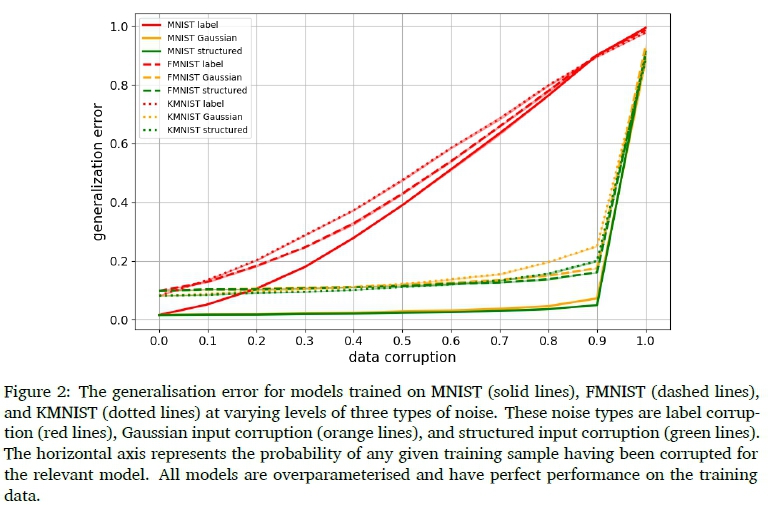
In order to investigate the sample sets and activation/weight vector interactions, several MLPs, containing 10 hidden layers of 512 nodes each, are trained on varying levels of noise. A standard experimental setup is used, as described in Appendix A. Figure 2 shows the resulting performance of the different models, when tested on uncorrupted test data. All models were able to easily fit the noisy training data, corroborating the findings of (Zhang et al., 2017).

Notice that, when analysing label corruption, there is a strong inverse correlation between the amount of label noise and the model's ability to generalise to unseen data. This suggests that either:

1. the models are memorising sample-specific input-output relationships and a certain portion of the unseen data is similar enough to a corresponding portion of uncorrupted training samples to facilitate appropriate generalisation; or

2. the global approximated function is somehow compartmentalised to contain fundamental rules about the task in some regions and ad hoc rules with which to correctly classify the corrupted samples in other regions.

Observe from the results of the two input corruptions ("Gaussian" and "structured") that noise in the input data has an almost negligible effect on generalisation up to the point where there is an insufficient amount of true data in the set with which to learn. This threshold is expected to change with more difficult classification tasks (more class variance and overlap), data sets containing fewer samples in total, and models with less parameter flexibility. This robustness to noise in the input space was not mentioned in (Zhang et al., 2017). We expect that is because the relevant experiments were aimed at showing that the models are large enough to memorise absolute input noise easily and still generalise from noiseless training data without considering the ability to generalise in the presence of noise.

The fact that input noise does not result in a linear reduction in generalisation ability still supports both the previous propositions. If the first postulate is true, then the samples with corrupted input data are memorised, but no samples in the evaluation set are similar enough to them to incur additional generalisation error. If the second postulate is true, then the regions in the approximated function that were determined by the corrupted input samples are simply never used for classifying the uncorrupted evaluation set.

It is also worth noting that the Gaussian and structured input corruptions have very similar influence on generalisation. The models are therefore able to generalise in the presence of input noise regardless of whether the corrupted samples have informative class-related structures in the input space.

4.2 Cosine similarities

The cosine similarity (cos 9 in Eq. 3) can be used as an estimate of how much the representation of a sample in a preceding layer is directionally similar to that of the set of samples for which a node tends to be active. By measuring the average cosine similarity of samples in a node's sample set with regards to the determinative weight vector (wⁱ_lin Eq. 3) and averaging over nodes in a layer, it is possible to identify layers where samples tend to be grouped together convincingly. That is, the samples are closely related (in the preceding feature space) and the resulting activation values tend to be large. Using Eq. 3, the mean cosine similarity per layer l (over all weight and active sample pairs at every node) can be calculated as

where N_lis a set of all the nodes in layer l and A_i is a set of all positive activation values at node i. Dead nodes (nodes that are not activated for any sample) are omitted when performing any averaging operations presented in this section. A dead node does not contribute to the global function and merely reduces the dimensionality of the feature space in the corresponding layer by one.

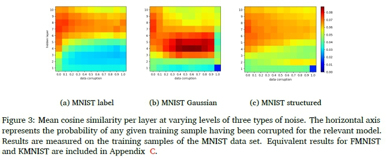
Figure 3 shows this metric for models trained on various amounts of noise. It can be observed that, in general, earlier layers tend to have lower sample set cosine similarities than later layers. This effect is amplified with any form of data corruption. It appears that label corruption results in the depth at which high mean cosine similarities are obtained being deeper in the noise-corrupted networks compared to the baseline models, while Gaussian input corruption results in the opposite. The effects of structured input corruption are much more subtle than the other two types of noise. These findings suggest that the coherence of input features of training data noise plays an important part in the depth at which a convincing representation of sample information is formed.

4.3 Sample set corruption composition

The noise in the data sets is introduced probabilistically on a per sample basis (see Algorithm 1 to 3). This provides a convenient way to investigate the composition of sample sets with regards to noise. Figure 4 shows how sample sets can consist of different ratios of true and corrupted sample information.

We define the polarisation of a node for a class as the amount the sample set of a node i favours either the corrupted or uncorrupted samples of a class c, respectively. This is defined as follows:

where A^c_iis a set of all positive activation values at node i in response to samples from class c, and A^c_iis a corresponding set limited to corrupted samples. By averaging over nodes and classes, a per-layer mean polarisation values can be obtained with the following equation:

where K is a set of all classes.

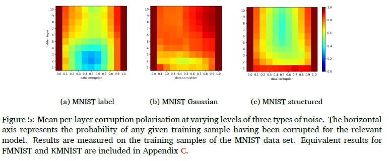
The polarisation metric indicates how much the sample sets formed within a layer are polarised between true class information and corrupted class information, for any given class. The relevant polarisation values are provided in Figure 5. The main observation is that sample sets tend to be highly in favour of true or corrupted sample information. This is especially prevalent for Gaussian input corruption where there is very little feature correlations to be found in the corrupted samples. The label corruption produces lower polarisation earlier in the model, but this is to be expected seeing as the input data has strong coherence based on correlations in class-related input structures. Again, we see that the structured input corruption does not greatly affect the change in sample information representation across depth. These findings support the second postulate in Section 4.1. It appears that sub-regions in the function space are dedicated to processing different kinds of training data.

4.4 Discussion

In this section we have shown that several overparameterised DNNs with no explicit regularisation are able to generalise well with evident spurious input-output relationships present in the training data. We have used empirically evaluated metrics to show that, in the presence of noise, well-separated per-node sample sets are generated later in the network compared to baseline cases with no noise. Additionally, these well-separated sets of samples are highly polarised between samples containing true task information and samples without.

If we adopt the viewpoint that nodes in hidden layers act as collaborating feature differentiators (separating samples based on feature criteria that are unique to each node) to generate informative feature spaces, then each layer also acts as a mixture model fitting samples based on their representation in the preceding layer. A key insight is that each model component is not fitted to all samples in the data set. Model components (referring to a node and its corresponding in-fan weight vector) are optimised on a specific subset of the population as determined by the activation patterns in the preceding layer. And, as we have observed, these subpopulations can and tend to be composed of true task information or false task information.

In this sense, some model components of the network are dedicated to correctly classifying uncorrupted samples, and others are dedicated to corrupted samples. To generalise this observation to training scenarios without explicit data corruption, it can be observed that in most data sets samples from a specific class have varied representations. Without defining some representations as noise, they are still processed in the same way the structured input corruption data is processed in this paper, hence the strong similarity between the baseline models and those containing structured input noise. This is also why it is possible to perform some types of multitask learning. One example would be combining MNIST, FMNIST, and KMNIST. In this scenario the training set will contain 180 000 examples with consistent training labels, but three distinct representations in the input space. For example, class 6 will be correctly assigned to the written number 6, a shirt, and a certain Japanese character.

To summarise, DNNs do overfit on noise, albeit in a benign fashion. The vast representational capacity and non-linearities enable sub-components of the network to be dedicated to processing sub-populations of the training data. When out-of-sample data is to be processed, the regions most similar to the unseen data is used to make predictions, thereby preventing the model components fitted to noise from affecting generalisation. In effect, contradictory training samples are separated from one another and modelled independently, each associated with more closely related samples, only if such samples exist. This ensures that (within reasonable bounds) neither noise nor the memorisation of a very large number of samples necessarily influence a given prediction. This sheds light on why excessive capacity does not necessarily lead to overfitting and a corresponding deterioration of generalisation. At least in the investigated framework, additional parameters means an increased number of sub-components with which to separate potentially detrimental feature descriptors from those that are related to the true underlying data distribution. These findings suggest that the capacity of a DNN should not be thought of as the complexity of the functions it will approximate but rather in its ability to partition data into signal and noise. This is akin to the processing of noise in a relational database, where attributes can have a varying number of possible values but an increased number of columns or rows will not result in less accurate responses to queries.

 

5 DOUBLE DESCENT AND LABEL CORRUPTION

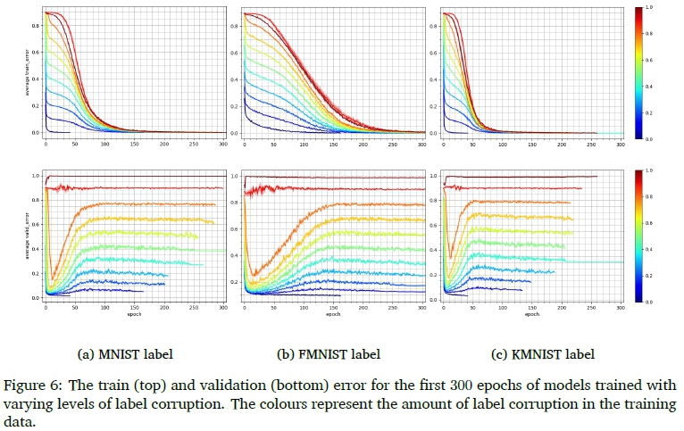
Figure 6 presents a phenomenon observed during the training of models containing label corruption. Notice that there is an initial period of very good generalisation before performance starts deteriorating, after which the system converges on the final validation error and stabilises. The early generalisation performance is reminiscent of a classic U-shaped bias-variance trade-off curve, beyond which there is a slight improvement in performance near the point of interpolating the training data completely. This is especially visible for models with more uncorrupted than corrupted samples - see Appendix C for a clearer visual depiction. No such behaviour was observable for models including Gaussian- or structured input corruption.

This behaviour seems related to one aspect of the "double-descent" phenomenon that was first explicitly demonstrated in Belkin et al. (2018) for simple MLPs, decision trees, and random features, on a model-wise (varying model capacity) basis. Specifically, in Belkin et al. (2018) it was found that, under certain training conditions, if a machine learning algorithm's capacity is increased beyond the point that is necessary to completely interpolate the training data, generalisation performance improves. Later, Nakkiran et al. (2020) demonstrated the phenomenon for more complex models, such as ResNet18 and some Transformer models, and highlighted a more general form of double descent: one that occurs both as a function of model capacity and training epochs. The mechanisms producing this phenomenon are still unclear and this is an active and important field of research, especially because of its stark contrast to classical notions of generalisation in machine learning (which expect excess capacity to uniformly impede generalisation).

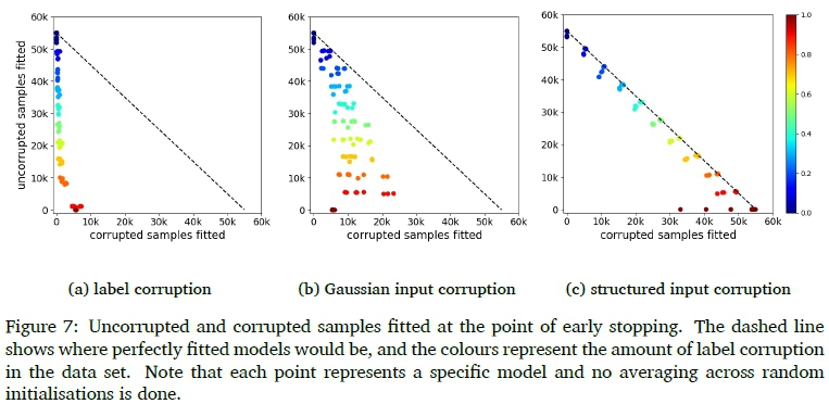
Within the context of this paper all ability of a model to generalise to the validation or test set can be attributed to feature descriptors learned from uncorrupted samples. It is then a natural question to ask whether the set of samples fitted at the point of peak performance are wholly uncorrupted, thereby allowing good generalisation. Figure 7 provides a scatter plot depicting the fitted training samples at the point of early stopping. Each model was trained for 50 epochs and early stopping was used to obtain the model at the point of peak performance. Notice that the models do not fit corrupted samples and uncorrupted samples equally under the effects of early stopping. These results indicate that our models fit uncorrupted samples first. Additionally, take note that virtually all the uncorrupted samples are fitted at the point of early stopping and, even at 100% label corruption, only a small fraction of the corrupted training data has been fitted at this early stage of training.

With these results in mind, we present the following conjecture to explain the presented epoch-wise double-descent phenomenon.

DNNs fit easier samples first. These samples share input feature structures that the gradient descent based optimisation process can take advantage of. When these samples have been fitted, and assuming sufficient model capacity, the remaining samples are fitted up to near the point of interpolation (0.0 training error). Beyond this point a representation has been obtained that fits most training samples and generalisation can improve slightly by means of classical empirical risk minimisation (depending on the ratio of easier and harder samples).

The notion of a DNN learning simple patterns before memorising noise is not new. It was already suggested in Arpit et al. (2017) and Rahaman et al. (2019). The novelty in our proposition is in using it as a lens to account for the epoch-wise double descent.

The conjecture can also explain why there is no double-descent for models containing structured input corruption. The corrupted samples are still easy to fit, based on the definition provided above. As for Gaussian input corruption, these corrupted samples are definitely hard to fit, however based on the behaviour explained in Section 4.4, they are too dissimilar to the uncorrupted samples to have an effect on the weight vectors fitted to uncorrupted samples.

 

6 CONCLUSION

We investigated the phenomenon that overparameterised DNNs are able to generalise in spite of perfectly fitting noisy training data. We studied fully-connected feedforward networks in the presence of different types of noise, and found that the ability of these networks to generalise is a direct result of the modular way in which training samples are fitted during optimisation. Our main conclusions are summarised below.

• Per sample input noise that is sufficiently different to the true data distribution has negligible effects on generalisation, provided enough representational capacity. This is in contrast with per sample label noise that increases test error in direct proportion to the noise level, with the network retaining classification accuracy in proportion to the uncorrupted samples that remain in the training data.

• Networks are able to ignore noise in the first case (input noise), since sub-units of ReLU-activated MLPs are fitted to sub-populations of the training set based on local similarity. Specifically, individual nodes tend to activate for noise or true data, rather than a combination of both. This means that features learnt from corrupted samples have no effect on noiseless test results.

• The same effect is at play in the second case (label noise), with correct samples processed separately from the label-corrupted versions, but with all sub-components triggered during the evaluation process.

• From this perspective, additional parameters therefore imply an increased number of sub-components with which to separate potentially detrimental feature descriptors from those that are related to the true underlying data distribution.

• In addition, we demonstrate that DNNs fit uncorrupted training data first, which fits our conjecture that easier samples are in general fitted first. Early in the training process, the model mainly fits uncorrupted samples, resulting in a low test error. Error increases as corrupted samples start influencing model behaviour. This provides a direct explanation for the phenomenon referred to as epoch-wise double descent, in the presence of low to moderate levels of label corruption.

Future work will continue to work towards a formal framework with which to characterise the collaborating sub-components and, based on this, further investigate more theoretically grounded predictors of generalisation. It would also be prudent to further investigate our conjecture with regards to double-descent, in order to gain further insight into the more general phenomenon.

 

References

Arpit, D., Jastrzebski, S., Ballas, N., Krueger, D., Bengio, E., Kanwal, M. S., Maharaj, T., Fischer, A., Courville, A. C., Bengio, Y. & Lacoste-Julien, S. (2017). A closer look at memorization in deep networks. International Conference on Machine Learning.

Belkin, M., Hsu, D., Ma, S. & Mandal, S. (2018). Reconciling modern machine learning and the bias-variance trade-off. ArXiv, abs/1812.11118.

Chaudhari, P., Choromanska, A., Soatto, S., LeCun, Y., Baldassi, C., Borgs, C., Chayes, J. T., Sagun, L. & Zecchina, R. (2017). Entropy-SGD: Biasing gradient descent into wide valleys. International Conference on Learning Representations.

Clanuwat, T., Bober-Irizar, M., Kitamoto, A., Lamb, A., Yamamoto, K. & Ha, D. (2018). Deep learning for classical Japanese literature. ArXiv, abs/1812.01718.

Davel, M. H. (2019). Activation gap generators in neural networks. South African Forum for Artificial Intelligence Research, 64-76.

Davel, M. H., Theunissen, M. W., Pretorius, A. M. & Barnard, E. (2020). DNNs as layers of cooperating classifiers. Association for the Advancement of Artificial Intelligence. https://doi.org/10.1609/aaai.v34i04.5782

Dinh, L., Pascanu, R., Bengio, S. & Bengio, Y. (2017). Sharp minima can generalize for deep nets. International Conference on Machine Learning.

Elsayed, G. F., Krishnan, D., Mobahi, H., Regan, K. & Bengio, S. (2018). Large margin deep networks for classification. Conference on Neural Information Processing Systems.

Frankle, J. & Carbin, M. (2019). The lottery ticket hypothesis: Finding sparse, trainable neural networks. International Conference on Learning Representations.

Gale, T., Elsen, E. & Hooker, S. (2019). The state of sparsity in deep neural networks. ArXiv, abs/1902.09574.

Glorot, X., Bordes, A. & Bengio, Y. (2011). Deep sparse rectifier neural networks. International Conference on Artificial Intelligence and Statistics.

Goodfellow, I., Bengio, Y. & Courville, A. (2016). Deep learning. MIT Press.

He, K., Zhang, X., Ren, S. & Sun, J. (2015). Delving deep into rectifiers: Surpassing human-level performance on imagenet classification. IEEE International Conference on Computer Vision, 1026-1034. https://doi.org/10.1109/ICCV.2015.123

Hochreiter, S. & Schmidhuber, J. (1997). Flat minima. Neural Computation, 9, 1-42. https://doi.org/10.1162/neco.1997.9.1.1        [ Links ]

Jastrzebski, S., Kenton, Z., Ballas, N., Fischer, A., Bengio, Y. & Storkey, A. J. (2019). On the relation between the sharpest directions of DNN loss and the SGD step length. International Conference on Learning Representations.

Jiang, Y., Krishnan, D., Mobahi, H. & Bengio, S. (2019). Predicting the generalization gap in deep networks with margin distributions. International Conference on Learning Representations.

Kawaguchi, K., Kaelbling, L. & Bengio, Y. (2017). Generalization in deep learning. ArXiv, abs/1710.05468.

Keskar, N. S., Mudigere, D., Nocedal, J., Smelyanskiy, M. & Tang, P. T. P. (2017). On large-batch training for deep learning: Generalization gap and sharp minima. International Conference on Learning Representations.

Krueger, D., Ballas, N., Jastrzebski, S., Arpit, D., Kanwal, M. S., Maharaj, T., Bengio, E., Fischer, A. & Courville, A. C. (2017). Deep nets don't learn via memorization. International Conference on Learning Representations.

LeCun, Y., Bottou, L., Bengio, Y. & Haffner, P. (1998). Gradient-based learning applied to document recognition. Proceedings of the IEEE, 86(11), 2278-2324. https://doi.org/10.1109/5.726791        [ Links ]

Li, H., Xu, Z., Taylor, G., Studer, C. & Goldstein, T. (2018). Visualizing the loss landscape of neural nets. Conference on Neural Information Processing Systems.

Loroch, D. M., Pfreundt, F.-J., Wehn, N. & Keuper, J. (2018). Sparsity in deep neural networks - An empirical investigation with TensorQuant. ArXiv, abs/1808.08784. https://doi.org/10.1145/3146347.3146348

Maurer, A. & Pontil, M. (2012). Structured sparsity and generalization. Journal of Machine Learning Research, 13, 671-690.         [ Links ]

Montufar, G. F., Pascanu, R., Cho, K. & Bengio, Y. (2014). On the number of linear regions of deep neural networks. Advances in neural information processing systems 27 (pp. 29242932). Curran Associates, Inc.         [ Links ]

Nakkiran, P., Kaplun, G., Bansal, Y., Yang, T., Barak, B. & Sutskever, I. (2020). Deep double descent: Where bigger models and more data hurt. International Conference on Learning Representations.

Neal, B., Mittal, S., Baratin, A., Tantia, V., Scicluna, M., Lacoste-Julien, S. & Mitliagkas, I. (2018). A modern take on the bias-variance tradeoff in neural networks. ArXiv, abs/1810.08591.

Neyshabur, B., Bhojanapalli, S., McAllester, D. & Srebro, N. (2017). Exploring generalization in deep learning. Conference on Neural Information Processing Systems.

Novak, R., Bahri, Y., Abolafia, D. A., Pennington, J. & Sohl-Dickstein, J. (2018). Sensitivity and generalization in neural networks: An empirical study. International Conference on Learning Representations.

Raghu, M., Poole, B., Kleinberg, J., Ganguli, S. & Sohl-Dickstein, J. (2017). On the expressive power of deep neural networks. International Conference on Machine Learning, 28472854.

Rahaman, N., Baratin, A., Arpit, D., Dráxler, F., Lin, M., Hamprecht, F. A., Bengio, Y. & Cour-ville, A. C. (2019). On the spectral bias of neural networks. International Conference on Machine Learning.

Shalev-Shwartz, S. & Ben-David, S. (2014). Understanding machine learning: From theory to algorithms. Cambridge University Press. https://doi.org/10.1017/CBO9781107298019

Sun, S., Chen, W., Wang, L. & Liu, T. (2015). Large margin deep neural networks: Theory and algorithms. ArXiv, abs/1506.05232.

Theunissen, M. W., Davel, M. H. & Barnard, E. (2019). Insights regarding overfitting on noise in deep learning. South African Forum for Artificial Intelligence Research, 49-63.

Vapnik, V. (1999). An overview of statistical learning theory. IEEE Transactions on Neural Networks 1999, 10 5, 988-99. https://doi.org/10.1109/72.788640        [ Links ]

Xiao, H., Rasul, K. & Vollgraf, R. (2017). Fashion-MNIST: A novel image dataset for benchmarking machine learning algorithms. ArXiv, abs/1708.07747.

Zhang, C., Bengio, S., Hardt, M., Recht, B. & Vinyals, O. (2017). Understanding deep learning requires rethinking generalization. International Conference on Learning Representations.

 

 

Received: 08 May 2020
Accepted: 05 October 2020
Available online: 08 December 2020

 

 

A EXPERIMENTAL SETUP

The classification data sets that are used for empirical investigations are MNIST (LeCun et al., 1998), FMNIST(Xiao et al., 2017), and KMNIST(Clanuwat et al., 2018). These data sets are drop-in replacements for each other, meaning that they contain the same number of input dimensions (28 x 28, 784 flattened), classes (10), and examples (70 000). In all training scenarios a random split of 55 000 training examples, 5 000 validation examples, and 10 000 evaluation examples are used. The generalisation error is measured on the evaluation set. 293 out of the 297 models attained a training error of 0.0. The four exceptions all had a training error smaller than 0.00005.

All models are trained for 1 500 epochs or up to the point of interpolation, whichever occurs first. Model weights are initialised with the He initialisation scheme (He et al., 2015). Randomly selected mini-batches of 64 examples are used to calculate losses. A fixed MLP architecture containing 10 hidden layers of 512 nodes each is used, with a single bias node at the first layer. ReLU activation functions are used at all hidden layers. A standard SGD optimiser is used with a cross entropy loss function. The learning rate is set to 0.01 at initialisation and multiplied by a factor of 0.99 every 10 epochs. No output activation function is employed and no additional regularising techniques (batch normalisation, weight decay, drop out, data augmentation, and early stopping) are implemented.

 

B ALGORITHMS FOR ADDING NOISE

The first type of noise is identical to the "partially corrupted labels" in (Zhang et al., 2017) except for the selection of alternative labels. Instead of selecting a random label uniformly, we select a random alternative (not including the true label) uniformly. This results in a data set that is corrupted by exactly the probability value P that determines corruption levels (see Algorithm 1). The second type of noise is similar to the "Gaussian" in Zhang et al. (2017), with the difference being that instead of replacing input data with Gaussian noise selected from a variable with identical mean and variance to the data set, we determine the mean and variance of the Gaussian in terms of the specific sample being corrupted, as in Algorithm 2. In other words, the corrupted sample contains features that are sampled from a Gaussian distribution that has a mean and standard deviation equal to those of the features of the uncorrupted sample. The third type of noise replaces input data with alternatives that are completely different to any in the true data set but still structured in a way that is predictable. This is accomplished by rotating the sample 90° counter-clockwise about the centre (prior to flattening the image data), followed by an inversion of the feature values. Inversion refers to subtracting the feature value from the maximum feature value in the sample - see Algorithm 3.

 

C ADDITIONAL RESULTS

The mean cosine similarities and mean polarisation values for analyses conducted on the FM-NIST and KMNIST data sets are provided in Figure 8 and 9, respectively. Notice that the same observations can be made when compared to the MNIST results in Section 4.2 and 4.3. It is, however, worth noting that for a classification task with more overlap in the input space such as FMNIST, the well-separated sample sets are generated at even later layers.

 

 

 

 

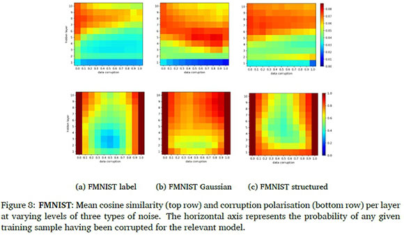
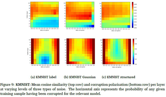
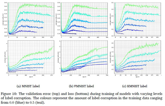
Figure 10 shows the per-epoch validation errors and losses for models with label corruption ranging from 0.0 to 0.5. These curves clearly show a slight improvement in generalisation during the second descent in the validation error. Take note that, interestingly, there is no second descent in the per-epoch loss curves. This suggests that, during the second descent, appropriate decision rules are learned for a portion of the validation set, however, this is at the cost of an extreme increase in loss values for another portion.