An Android Application-based Surface Oust Classifier

 

 

P. Dabee; B. Rajkumarsingh; Y. Beeharry

Department of Electrical and Electronic Engineering University of Mauritius, Réduit, Mauritius. Email: dabeepreetiksha@gmail.com; b.rajkumarsingh@uom.ac.mu; y.beeharry@uom.ac.mu

 

 

---

ABSTRACT

Surface dust can be a source carrier of viruses, bacteria and air pollution which entail common health issues such as asthma attacks, chest tightness, wheezing and difficulty in breathing. Visually perceived, cleanliness is one measure of indoor air quality and is the subjective assessment of cleaning quality. The aim of this work is to use pattern recognition mediated through a mobile application to analyse and classify dust in households, in order to obtain useful information about the dust sources for the selection of appropriate countermeasures in view to improve air quality and better manage the cleaning of indoor surfaces. The dust type categorization in this work are pollen, rock and ash. This paper also explores the concept of transfer learning techniques and adopts it for small particle classification using CNN models by developing a surface dust application for android smartphones. The behaviour of InceptionV2, InceptionV3, ResNetV2, MobileNetV2 and MobileNetV3 as dust feature extractors were analysed based on their accuracy, precision, recall and Fl-Scoreperformance metrics. Results show that MobileNetV3 model is best suited as a dust feature extractor and rapid dust prediction with an accuracy of up to 92% and low-size storage of only 30 megabytes.

Additional Keywords: Android; Classification; Transfer Learning; Smartphone; Surface dust.

---

 

 

1 Introduction

People in developed countries spend over 90% of their time indoors, making indoor air quality one of the most serious environmental issues [1,2]. They may be exposed to a wide range of pollutants generated from various indoor and outdoor sources during this time [3], as the level of indoor particles is dependent on the particles generated within indoor spaces and in the surrounding environment [4], Buildings' open windows, doors and ventilation systems are the primary sources of external infiltration into the internal environment [5]. As a result, it's critical to describe and identify indoor and outdoor dust sources. Dust is a detritus comprising a mixture of indoor and outdoor pollutants and its particles can range from small invisible sizes to relatively large visible sizes (1 μm to 100 μm) which under the impact of gravity, settle down on surfaces [6,7]. Several studies have been undertaken to characterize dust in indoor environments. In [8], the results of the characterization of settled dust particles are presented in various indoor micro-environments of Brazilian universities. In [9], a comparison of thirty air-conditioned and naturally ventilated classrooms in Brazilian colleges are made to assess indoor air quality. The relationship between dust and office surfaces are discussed in [10]. In detail, indoor and outdoor exposure to dust is one cause of non-communicable diseases such as myocardial infection, ischemia, chronic obstructive pulmonary disease, stroke and cancer [11, 12, 13, 14]. According to the findings, a number of dust occurrences were substantially linked to changes in asthma severity [15, 16, 17, 18].

Existing dust detection systems are mainly acquired from dust sensors using optical measurement techniques. Its working principle is based on the attenuation of light intensity during penetration of a beam on the dusty surface by absorption and dispersion. Dust sensors use this principle to determine the dust concentration by the intensity of the received beam. Dust meters also use this technique to determine PM2.5 and PM10 particles (particulate matter 2.5 and 10 microns) in the air [6, 11].

To the best knowledge of the authors, there is no earlier mobile applications of the individual Machine Learning (ML) models utilized here to the classification of indoor dust, despite their great performance in prediction and spatial modelling of natural hazards. Most of the ML methods have been used for dust storm detection. The detection of dust storms using probabilistic multispectral image analysis has been investigated [19]. A Maximum Likelihood classifier and a Probabilistic Neural Network (PNN) to automate the dust storm identification process using this feature set were created. The authors of [20, 21] have recently proposed two ensemble and integrated models to map the source of the dust storm. The authors investigate the Jazmurian Basin's vulnerability to dust emissions using six machine-learning algorithms (XGBoost, Cubist, BMARS, ANFIS, Cforest and Elasticnet). Cforest was found to have the best results. According to [21], dust source modelling and prediction can be performed using hybridized neural fuzzy ensembles. Using quantitative computed tomography-based airway structural and functional data, an artificial neural network (ANN) model was used for identifying cement dust-exposed (CDE) patients [22].

Although there is no current work being done in the field of dust classification using a smartphone, the use of CNN on smart phones to detect and categorize diverse image datasets is still ongoing. The authors of [23] put forward a skin cancer classification model using ResNet architecture with a final prediction accuracy of 77%. The authors of [24], presented a work for brain tumour classifications using CNN architecture based on MRI images acquired online. The authors of [25], adopted the MobileNetV2 architecture and transfer learning approach for the development of a flower classifier which managed to achieve 96% correct predictions for all 5 flower classes. The author of [26] proposed the InceptionV3 model for the classification of human face shapes. This technique was based on the training the last layers from a pre-trained InceptionV3 model with a model performance of 84%. The major issue for training large CNN models from scratch is the unavailability of big training datasets. Nevertheless, even with a small dataset, a reliable classifier may be created with a very good prediction result. This may be accomplished by using models that have been pre-trained on a large dataset from a similar domain.

There is still no existing application for the detection of relatively small particles, using an android camera which is the most practical, readily available and affordable device of this modern era. As a result, this work explores the concept of transfer learning techniques and adopts it in the field of cleaning for small dust particles detection to build a dust application all through a mere smartphone camera. This application can be used by everyone including the ageing population to accurately detect unclean surfaces and the dust content lying on these surfaces. As such, immediate actions can be taken to monitor cleanliness at one's fingertips. Additionally, there is a significant health and safety benefit to the proposed method in industries where a lot of dust is present. For example, in a coal mine and cement factory, the technology be used to monitor the dust quality at regular intervals; the dust (amount and type) on a certain surface and then make an alarm if it exceeds safe levels.

This paper investigates the behaviour of InceptionV2, InceptionV3, ResNetV2, MobileNetV2 and MobileNetV3 as dust feature extractors based on their accuracy, precision, recall and Fl-Score performance metrics. The images of surface dust were acquired by clicking photos of ash dust, rock dust and pollen dust under different lighting conditions and surfaces, trained and subsequently converted to be deployed in related devices.

The rest of this article is organized as follows. In Section 2, an overview of the image-based surface dust classification and the surface dust android application is illustrated. A brief review of the fundamental CNN architecture, transfer learning and its methods is presented in Section 3. The experimental research is described in Section 4 and the results of the experiments are presented in Section 5. Section 6 brings the article to a close-by summarizing the conclusions of the analysis.

 

2 Image-Based Surface Dust Classification

2.1 Surface Dust Classifier

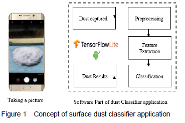
Figure 1 illustrates the basic process of the surface dust classifier. Firstly, the user captures the surface dust image. Then, the image is resized and placed into an image view. The dust model extracts the features associated with each dust type i.e., pollen dust, ash dust and rock dust. It recognizes the features that were learned during its training phase and performs the classification. The dust result along with the prediction accuracy is displayed on the top of the image view with an indication of the amount of dust lying on the surface.

 

 

2.2 Surface Dust Android Application

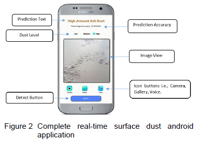
Figure 2 illustrates the final real-time surface dust application with a set of achieved objectives such as good surface dust prediction accuracy with an indication of the amount of dust lying on a specific surface, a small application size of 30 MB, user-friendly interface with iconized buttons. The application also comes with voice output communication aids integration for its general use including the aging population.

 

 

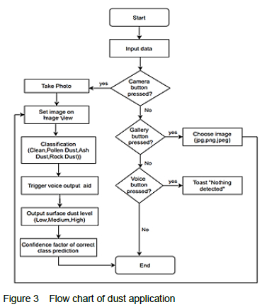
Once the image file and corresponding labels are converted, they are downloaded for further adjustments in the android studio platform. Figure 3 depicts the essential functions of the application that needs to be conducted on android studio towards achieving the final result.

 

 

3 Convolutional Neural Network

CNNs as shown in [19], is the most common type of deep neural network best suited for computer vision tasks. Its architecture was designed in such a way that it minimizes the number of parameters fed at the input layer even if the image size increases, reducing computational cost, power and memory requirements. CNNs get as input an image in the form of matrices e.g. (224,224,3) where the first two parameters are length and width in terms of pixels and the third parameter describes the image property (RGB colour image) [27]. In the convolution layer [28], a convolutional filter is applied which slides over the original image to produce a new featured map known as the convolved feature [29]. The max pooling layer [30] reduces the dimensions of the feature map to minimize the number of parameters while preserving as many images as possible. Fully Connected layers are part of the last few layers of the neural networks. The layers are said to be fully connected when every neuron of the first layer is connected to one of the second layers [31].

3.1 Transfer Learning and Feature Extraction

Transfer learning [32] is a technique that utilizes a neural architecture which has already been trained on some other problems and transfers all or part of the acquired knowledge to a new model to solve a different type of problem. Transfer learning greatly reduces the number of parameters used for training a model from scratch by adopting some pre-used extracted features from previous training [33]. Feature extraction is a portion of the training product of a model. It consists of the high-level layer where the mapping of the input is done for final classification. This approach further reduces the number of parameters from a pre-trained model to solve a new custom problem [34]. In this approach, only the fully connected layer which is added to the new model is to be trained after loading the pre-training weights. This process is known as model Fine-Tuning.

 

4 Experimental Study

In this work, we have trained surface dust classifiers using: I. A CNN dust model trained from scratch and one trained with a transfer learning approach.

II. The pre-trained models InceptionV2, InceptionV3, ResNetV2, MobileNetV2, MobileNetV3 as dust features extractors.

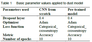
A comparative study was done based on accuracy, training time, model size, convergence rate and performance metrics to determine the best model adapted to the custom surface dust dataset. Finally, the optimal dust model was chosen and subsequently converted into a Flatbuffer file extension (.tflite) through the TensorFlow Lite Converter API. The optimized Flatbuffer allows conversion with minimal accuracy loss and operates efficiently on mobile phones with less computational and memory requirements [35]. In both strategies, techniques such as data augmentation, dropout layer, early stopping and use of a validation dataset were incorporated to prevent model overfitting. Table 1 shows the basic parameters values adopted for the implementation of the dust model.

 

 

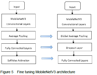
4.1 MobileNetV3

MobileNet is a form of CNN devised for mobile vision applications. MobileNet is a lightweight, low-powered, accurate and low-latency model. The architecture of MobileNetV3 is based on separable depth wise and pointwise convolutions [36]. The depth wise layer is used to filter the input channels while the pointwise layer is used to combine the filtered inputs to create new features. In normal convolutions, the filtering and combining input map features were done in a single layer which resulted in unnecessary and complex mathematical operations with the end classification being less accurate. As such, the MobileNetV3 architecture reduces the complexity of multiplications up to nine times when compared with a standard convolution performed in traditional CNN networks [12] adapted for image-related tasks [37].

Feature extraction is the backbone for object classification or detection [38]. The accumulations of features of an image, collectively known as feature vectors are used to categorize the objects. Feature extractor models map image pixels into their feature space [39]. The convolution layers can now just pass on these features from the pre-trained weights. The entire model does not need to be trained again; the only modifications lie on the last three layers of the model. The input fed in the model is an RGB image with 224 χ 224 pixels comprising 3 channels. From figure 5, the Average Pooling, FC and SoftMax layers are deleted from the original architecture and the Global Average Pooling (GAP), Dropout and Fully Connected (FC) layers are added to fit/tune the new model to our custom dust dataset.

 

 

4.1.1 Global average pooling layer

The GAP layer further diminishes the total model parameters resulting in faster computations and reduces overfitting of the data.

4.1.2 Dropout layer

The Dropout layer is a technique used to prevent the model from overfitting. It is known as a regularization method [33] where random neurons are ignored during the training phase.

4.1.3 Fully-connected layer

The FC layers finally connect all the other layers. It is the flatten matrix that goes through the FC layer leading to the final prediction at the output layer.

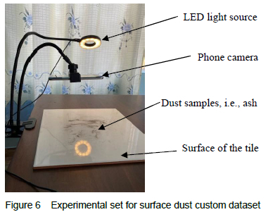
4.2 Experimental Setup

Figure 6 illustrates the image acquisition process. The image acquisition process was conducted during the daytime using tiles of uniform dimensions 30cm χ 30cm. The tiles acted as a surface where the pollen, ash and rock dust were spread to mimic dust deposits. All the data were accumulated using real dust originating from ash and rock. Instead of real pollen dust, which is difficult to acquire, dust originating from a plant source having a similar grainy texture and colour as pollen dust was used.

 

 

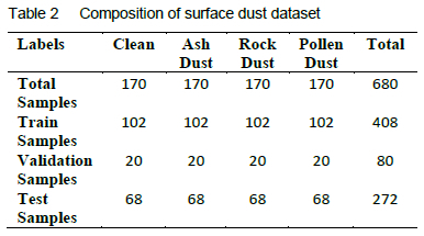
The custom dataset is partitioned into the training set and the validation set where 60% of data is used for training, 20% as cross-validation data and 20% as testing data. This partitioning ratio is common to cater for an unbalanced small dataset with the aim to improve model effectiveness and accuracy [40]. Table 2 below shows the composition of the small custom dust dataset.

 

 

4.2.1 Hardware and Software Requirements

The basic requirement for the dust detection application is a smartphone with a camera. The android camera being used in this experiment is 12 Megapixels. The minimum requirement for machine learning processes is NVIDIA GPUs [41]. GPU-accelerated deep learning process decreases the training waiting time especially if models are being trained for large datasets. All machine learning processing was done in the cloud platform (Jupyter Notebook) due to the free availability of GPU and storage.

4.3 The Dataset

The dataset is based on images of surface dust which will be captured using the rear android camera. The dataset comprises 4 classes namely: Clean, Pollen Dust, Ash Dust and Rock Dust. Figure 7 depicts the creation of a dust dataset intending to increase the variety of the dust images leading to a more robust dataset. Among them are:

 

 

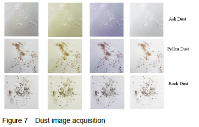
• Dust acquisitions images from projecting yellow, blue and white light sources.

• Dust acquisitions images of varying light intensities of the light source: 100%, 75%, 50% and 25% of the highest capability of the LEDs. 100% capacity of light source corresponded to the range. 1000 to 1200 Lux, 75% capacity of light source to 700 to 800 Lux, 50% capacity of light source to 300 to 500 Lux and 25% capacity of light source to 100 to 250 Lux. The variation of light intensity can be observed in figure 7 from left to right.

• Dust acquisition images by varying the position of the light source i.e., 10, 15, 25, 30 degrees with respect to the normal of the dust sample.

• Dust acquisition images by varying the distance of the camera from the dust samples. The distances ranged from close focus (4 cm close to dust deposit) to 35 cm (maximum distance reached due to camera resolution. For distances higher than 35 cm dust lying on the surfaces could not be observed properly.

• Dust acquisition images by changing the spread orientation and amount of dust sprinkle deposited under the different lighting conditions. The amount of dust sprinkle/spread on the surface was done in a random way ranging from little sprinkle (covering small tile area) to large layered dust deposit (occupying large surface area). The spread was also oriented differently by rotating the tile for more dust spread variations. Dust spread was sprinkled to vary between 1 to 100% of the plate area.

4.4 Data Pre-processing

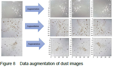
Data pre-processing is done using Keras Library. Its ImageGenerator function provides options such as zoom, rotate and flips added to the existing images to augment the dataset. This process minimizes the risk of over-fitting the model and it is useful where the dataset is small as a means to increase validation accuracy. The data augmentation technique is only applied to the training dataset. The original dataset is initially augmented by varying the light intensity, position of camera, distance of camera and spread of dust particles as mentioned previously. Further augmentation of the dataset is done using the zoom, rotate and flip options. Figure 8 shows the augmentation plots for the ash dust, pollen dust and rock dust training samples.

 

 

5 Results and Discussion

This section elaborated on the performance comparisons of traditional CNN model [12] and adoption of transfer learning approach, results of the five pre-trained models based on convergence rate, performance analysis metrics for image-based surface dust classification.

5.1 Training and Validation

From the learning curves of figure 9, the traditional CNN architecture [12] gave a rather worse performance compared to the one with the transfer learning approach. From the gap of the validation loss with the training loss learning curves, the model using transfer learning generalizes more than the model from scratch. It is noted that the gap between training loss and validation loss is small implying that the model is better at generalization on unseen data. The values obtained for the training accuracy, validation loss and training time for 10 epochs can be seen in table 3.

 

 

 

 

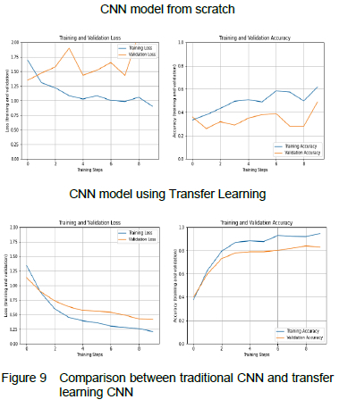
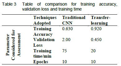
The maximum validation loss was obtained for traditional CNN. If the model from scratch is trained for the higher number of epochs, the model can achieve better accuracy with a high probability of model overfitting. The time it takes for transfer learning is approximately 4 times less than the traditional CNN approach. This is because of a reduced number of parameters that resulted in quick computations and more accurate results for the transfer learning approach.

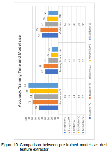
From figure 10, MobileNetV3 achieved an overall accuracy of 92% as compared to other models certainly due to its depth wise separable convolution approach. Its accuracy is approximately 4% higher than MobileNetV2. This is due to the further removal of unnecessary complex layers from the MobileNetV2 architecture resulting in better accuracy and faster computations in its version 3 architecture. InceptionV3 can also be a good choice due to its fair accuracy of 79% but its training time is high. This can be the cause of complex stacked layers of the inception model. InceptionV2 performed the worse among the others with the lowest accuracy of 60%. The ResNetV2 was a good competitor for the InceptionV3 model but was overcome in terms of accuracy for dust detection. The model size of MobileNet after compression was observed to be 30MB, the lowest among all the pre-trained models.

 

 

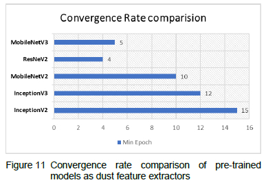
5.2 Convergence Rate

The convergence rate is a state where a model achieves a certain loss value where further training will not improve the model. The convergence rate is affected by factors such as model size, the complexity of the model and the training method used. It is seen in figure 11 that InceptionV2 achieved maximum validation accuracy at 15 epochs. The inception models are complex with many trainable layers therefore it takes more time to reach convergence. MobileNetV3 converges with a minimum epoch of 5. ResNet architectures are the fastest to converge at 4 epochs.

 

 

5.3 Performance Metrics

5.3.1 Dust model evaluation through classification report

Using the classification report function from the python Scipy library, metrics such as accuracy, precision, recall, specificity and F1-score including the macro and weighted average are calculated from its respective confusion matrix.

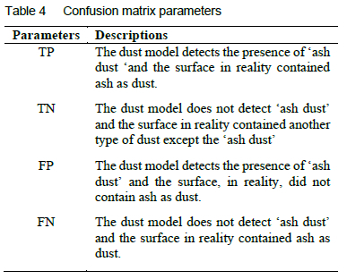
The confusion matrix consists of four scenarios namely True Positive (TP), True Negative (TN) and False Negative (FN) as given in table 4 for ash dust.

 

 

5.3.2 Accuracy

Accuracy gives the model's overall fraction of total samples correctly categorized by the classifier as in equation 1.

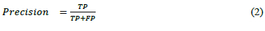
5.3.3 Precision

Precision is different from accuracy. It indicates what fraction of the positive predictions were actually correct. The higher the value of the precision metric, the better the dust model is performing. The formula for precision is given as in equation 2.

5.3.4 Recall or Sensitivity

Recall indicates the ratio of actual positives out of all positive samples the classifier accurately predicted as positive. It is also known as the True Positive Rate or sensitivity [42]. It is a metric for the classifier's ability to properly anticipate target outcomes that are related to the actual value. The higher the recall factor, the better the model is performing. Recall is calculated as in equation 3.

5.3.5 Specificity

Specificity is the opposite of recall. It gives the ratio of actual negatives out of all the negative samples that were correctly classified by the dust classifier. It is also named as True Negative Rate [42]. It is calculated as given in equation 4.

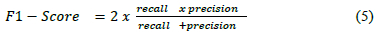
5.3.6 F1-Score

F1-Score is a combination of precision and recall. It is known as the harmonic mean of precision [30]. It is calculated as in equation 5.

5.3.7 Macro and Weighted Average

Macro averaging metrics are the unweighted mean average of precision, recall and Fl -score of each class label. It will perform the computation individually, that is by treating all the dust classes equally [43]. Weighted Average is a function that computes the probability score based on the proportion of each label in the dust dataset.

For analysing the effectiveness of the surface dust classifier, relying solely on accuracy classification can be delusive since we do not know what specific error the dust classifier has been making.

Table 5 shows the performance of the five pre-trained dust models based on different metrics such as precision, recall and Fl-score obtained from their respective confusion matrix.

 

 

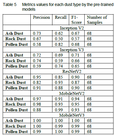
The number of samples of each class was 68. Since the dust dataset was a custom one, it was meticulously built by considering class imbalance factors to prevent biased classifications. From table 5, the dust model gave an overall good performance metrics for all dust types. MobileNetV3 is seen to be more precise with ash dust. MobileNetV2 gave a similar result to that of MobileNetV3 but seemed better performing with rock dust with 0.95 as the value for Fl-score. ResNetV2 was more sensitive to rock dust with similar Fl scores for the ash and pollen dust types implying a balance for both recall and the precision metrics. The iInceptionV3 gave the highest Fl-score for ash dust prediction while the inceptionV2 was able to better predict pollen dust. However, MobileNetV3 gave the best sensitivity of 1.00 for ash and pollen dust inferring FN predictions will be minimal for ash and pollen dust detection.

5.4 Testing Results

Eventually, after training the best pre-trained model was verified by using the test data for the prediction of the first set of elements on Jupyter Notebook. Table 6 shows the generalization accuracy for the first five test samples only with the maximum accuracy reaching close to 99.6% for the correct prediction of pollen dust type indicating that the MobileNetV3 was the optimal pre-trained model for correct classification of the surface dust.

 

 

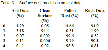
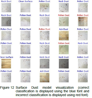
Figure 12 shows another visualization of the predictions obtained from the Mobile V3 dust model. Out of 30 test images displayed, only 4 images were wrongly predicted by the dust classifier. If we consider the 30 test images only, the model achieved an accuracy of 86.7% with up to 92% if larger test data were displayed. It can be observed there is a high variability in the results of the test set. This is specifically due to the combinations of different coverage percentages and different light intensities that have not been leaned by the machine learning model. This can be remedied by further increasing and augmenting the dataset used for the model training phase.

 

 

5.5 Testing of Dust Application on Android Device

5.5.1 Dust amount detection

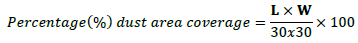
For this work, a tile of 30cm by 30cm was used throughout. The goal for this experimentation is to know whether the dust application is able to correctly determine the amount of dust based on the created threshold (low, medium and high). The method devised for determining the actual amount of dust in terms of area covered is shown in figure 13.

 

 

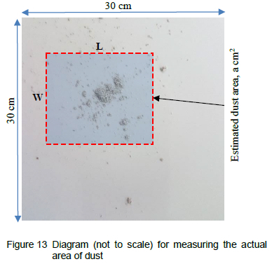
The dust area is estimated by calculated the L and W dimensions using:

 

 

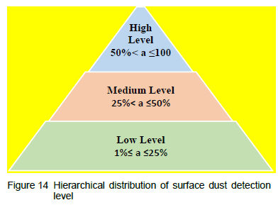
5.5.2 Dust level threshold

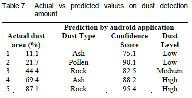
For the dust prediction through the application, a threshold was devised for categorization in terms of three dust levels as in figure 14. Thirty tests were conducted on unseen dust images to evaluate the accuracy of surface dust application by comparing the actual amount of dust in terms of area coverage as explained in the above section.

 

 

For simplicity, only five tests were shown as in table 7 with the predicted dust type, confidence score and level given by the dust classifier. Out of 30 tests, the model was able to correctly predict the amount of 28 dust samples.

 

 

5.5.3 Effect of varying camera distance from dust sample

The general trend, from figure 15, is a decrease in accuracy with an increase in distance, cm. The prediction accuracy at the minimum distance, 10 cm, is around 68%. At 15 cm height, the dust application observes a drastic increase of up to 74% in prediction accuracy. This is because, at a certain height, the field of view also increases which enhances prediction. This implies that the MobileNetV3 algorithm seems to better discriminate the dust features at an optimal wide field of view.

 

 

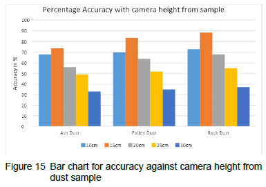
With increasing camera height from the dust sample, the dust classifier seems to correctly predict rock dust type compared to ash and pollen dust. This can be due to the size of rock dust. However, above 20cm the performance of the dust application decreases with smaller prediction accuracy percentages. The maximum height where the dust application can manage to detect dust is approximately 35cm above the dust sample but with an increased probability of wrongly predicted dust.

5.5.4 Testing dust model behaviour with surface colour and texture

This test was conducted using three different plain coloured tiles namely yellow, Gray, Blue and a textured tile. The camera height of 15 cm was fixed. The normal lighting conditions were used. The dust accuracy prediction given by the dust application is repeated 50 times to obtain an average for each type of tile investigated. The result obtained is shown in figure 16.

 

 

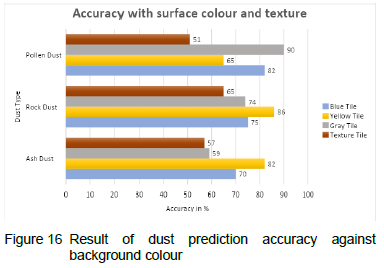
From figure 16, the dust application was able to correctly detect the presence of different dust types for both coloured and textured surfaces. For coloured surfaces, the grey tile as the background colour achieved the highest accuracy of 90% for pollen dust detection, yellow background with an accuracy of 86% for rock and 82% for ash dust detection. The model seems to perform better when there is a higher contrast between the foreground and the background colour. For instance, pollen dust being yellow provides a good distinction from the grey background. The ash and rock being darker in shades are more distinguishable from a pale-yellow background. For textured surfaces, the dust application gave an overall satisfactory accuracy above 50% for all dust types. The pollen dust detection seemed to be much affected with a textured surface. This may be because of its grainy-like appearance where the dust model may confuse with the background texture and the actual pollen dust.

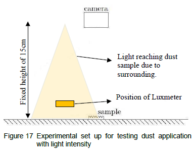
5.5.5 Testing dust model behaviour with light intensity of the surrounding.

The dust application was tested to see how the model behaved under the effect of external light intensity. Figure 17 shows the setup of the experiment. An android lux meter was used to measure the light intensity of the surroundings on an hourly daytime basis. A plain white tile was used to avoid any secondary effects on the accuracy values. The android camera height was fixed at 15 cm.

 

 

The mean value of the luminosity range obtained by the lux meter was taken. The graph of the prediction accuracy of each dust type with respect to intensity value is shown in figure 18.

 

 

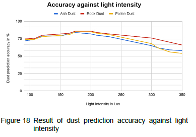
From the graph in figure 18. the external light intensity does not seem to have a major impact while categorising the dust types since the gap between their lines is small. A noticeable increase in dust prediction accuracy was observed at light intensities in the range of 170-200 lux for pollen dust, ash dust and rock dust. However, if the light intensity continues to increase, the percentage accuracy shows a decreasing slope. This implies that the dust classifier is at its best at optimal light intensity ranging from 170-200 lux. The decrease in accuracy can be due to the effect of extra brightness falling on the dust sample which affects the pixel values resulting in a more saturated image being captured by the camera. The dust details are more faded and hence difficulty is experienced by the dust classifier to correctly give a good confidence score for the respective dust classes.

 

6 Conclusion

The goal of this research is to use pattern recognition on a smartphone to analyze and classify dust inside, particularly in households, in order to gain some relevant information for the selection of countermeasures to be taken to enhance air quality and better manage household cleaning. MobileNetV3 architecture model proved to be the best-suited model as a dust feature extractor with an accuracy of 92%. fast training time and low sized model that classifies surface dust through a real-time dust vision application. During the training phase, the MobileNetV3 model was found to be 4% more accurate than MobileNetV2. Through the performance metrics analysis, the dust classifier seemed to be more efficient while classifying the ash dust amongst the other dust labels despite very good Fl-scores were also obtained for the other dust types. A captivating future work will be the creation of a dust dataset to recognize a wider range of dust for research on dust localization using powerful camera lenses. Another future work will be to test the dust application on different types of smartphones. with each having a different screen size and camera specifications. Alterations can also be made to the properties of the surface on which dust lies. e.g. colour, colour variations, texture and even geometry. Because the application is currently only available for android users, it could be expanded to include IOS devices in the future. This research could lead to low-cost surface dust monitoring devices in the food industry.

 

Contributions

Ms P. Dabee has worked on the dataset generation and development of CNN models as well as the android mobile application.

Dr. B. Rajkumarsingh has supervised Ms P. Dabee in the work and also worked on the paper write-up.

Dr. Y. Beeharry has reviewed and re-organized the paper as well as the referencing.

 

Lessons Learned

During the dataset creation phase, any type of background was used which was the main reason why the performances of the CNN models were lower. Thus, a major learning during the conduction of the work was that dataset creation for the training of the CNN models requires clean background in view to obtain more accurate predictions.

 

References

[1] United States Environmental Protection Agency. Science Inventory. URL https://cfpub.epa.gov/si/si_public_record_report.cfm?Lab=&dirEntrvId%C2%BC12464. 2022.

[2] L. Melymuk, H. Demirtepe, S. R. Jílková, Indoor dust and associated chemical exposures. Current Opinion in Environmental Science & Health, 15:1-6, 2020.

[3] A. P. Reis, C. Patinha, Y. Noack, S. Robert, A. C. Dias and E. F. da Silva. Assessing the human health risk for aluminium, zinc and lead in outdoor dusts collected in recreational sites used by children at an industrial area in the western part of the Bassin Minier de Provence, France. Journal of African Earth Sciences, 99(2):724-734, 2014.         [ Links ]

[4] J. L. Adgate, S. J. Mongin, G. C. Pratt, J. Zhang, M. P. Field, G. Ramachandran and K. Sexton. Relationships between personal, indoor, and outdoor exposures to trace elements in PM2.5. Science of the Total Environment, 386(1-3):21-32, 2007.         [ Links ]

[5] P. Singh, R. Saini and A. Taneja. Physicochemical characteristics of PM2.5: Low, middle, and high-income group homes in Agra, India-a case study. Atmospheric Pollution Research, 5(3):352-360, 2014.         [ Links ]

[6] M. L. Khadem and V. Sgarciu. Dust monitoring systems, in The Sixth International Conference on Systems and Networks Communications, Romania, 2011.

[7] X. Liu, M. R. Allen and N. F. Roache. Characterization of organophosphorus flame retardants' sorption on building materials and consumer products. Atmospheric Environment, 140:333-341,2016.         [ Links ]

[8] S. R. Jurado, A. D. P. Bankoff and A. Sanchez. Indoor air quality in Brazilian universities. International journal of environmental research and public health, 11(7):7081-7093,2014.         [ Links ]

[9] V. Sahu, S. P. Elumalai, S. Gautam, N. K. Singh and P. Singh. Characterization of indoor settled dust and investigation of indoor air quality in different micro-environments. International Journal of Environmental Health Research, 28(4):419-431, 2018.         [ Links ]

[10] J. Kildeso, J. Vallarino, J. D. Spengler, Η. S. Brightman and T. Schneider. Dust build-up on surfaces in the indoor environment. Atmospheric Environment, 33(5):699-707, 1999.         [ Links ]

[11]LevittSafety. How to measure dust in the workplace, URL http://www.levitt-safetv.com.

[12] World Health Organization. Health and the environment: addressing the health impact of air pollution. URL http://apps.who.int/gb/ebwha/pdf_files/WHA68/A68_ACONF2Revl-en.pdf. 2015.

[13] V. S. Chithra and S. M. S. Nagendra. Chemical and morphological characteristics of indoor and outdoor particulate matter in an urban environment. Atmospheric Environment, 77:579-587, 2013.         [ Links ]

[14] R. Goyal and P. Kumar. Indoor-outdoor concentrations of particulate matter in nine microenvironments of a mix-use commercial building in megacity Delhi. Air quality, atmosphere & health, 6:747-757, 2013.         [ Links ]

[15] J. L. Kim, L. Elfman, Y. Mi, M. Johansson, G. Smedje and D. Norbäck. Current asthma and respiratory symptoms among pupils in relation to dietary factors and allergens in the school environment. Indoor Air, 15(3):170-182, 2005.         [ Links ]

[16] K. Ueda, H. Nitta and H. Odajima. The effects of weather, air pollutants, and Asian dust on hospitalization for asthma in Fukuoka. Environmental health and preventive medicine, 15(6):350-357, 2010.         [ Links ]

[17] L. Thalib and A. Al-Taiar. Dust storms and the risk of asthma admissions to hospitals in Kuwait. Science of the Total Environment, 433(1):347-351, 2012.         [ Links ]

[18] P. Gupta, S. Singh, M. D. S. Kumar, M. Choudhary and V. Singh. Effect of dust aerosol in patients with asthma. Journal of Asthma, 49(2):134-138, 2012.         [ Links ]

[19] P. Rivas-Perea, J. G. Rosiles, Μ. I. C. Murguia and J. J. Tilton. Automatic dust storm detection based on supervised classification of multispectral data. Soft Computing for Recognition Based on Biometrics, 443454, 2010.         [ Links ]

[20] H. Gholami, A. Mohamadifar and A. L. Collins. Spatial mapping of the provenance of storm dust: Application of data mining and ensemble modelling. Atmospheric Research, 233:104716, 2020.         [ Links ]

[21] O. Rahmati, M. Panahi, S. S. Ghiasi, R. C. Deo, J. P. Tiefenbacher, Β. Pradhan, A. Jahani, H. Goshtasb, A. Kornejady, H. Shahabi, A. Shirzadi, H. Khosravi, D. D. Moghaddam, M. Mohtashamian and D. T. Bui. Hybridized neural fuzzy ensembles for dust source modeling and prediction. Atmospheric Environment, 224:117320, 2020.         [ Links ]

[22] T. Kim, W. J. Kim, C. H. Lee, K. J. Chae, S. H. Bak, S. O. Kwon, G. Y. Jin, Ε. K. Park and S. Choi. Quantitative computed tomography imaging-based classification of cement dust-exposed subjects with an artificial neural network technique. Computers in Biology and Medicine, 141:105162, 2022.         [ Links ]

[23] Β. Rokad and S. Nagarajan. Skin cancer recognition using deep residual network. URL https://arxiv.org/ftp/arxiv/papers/1905/1905.08610.pdf.

[24] T. Tazin, S. Sarker, P. Gupta, F. I. Ayaz, S. Islam, Μ. M. Khan, S. Bourouis, S. A. Idris and H. Alshazly. A robust and novel approach for brain tumor classification using convolutional neural network. Computational Intelligence and Neuroscience, 2021:2392395, 2021.         [ Links ]

[25] C. Narvekar and M. Rao. Flower classification using CNN and transfer learning in CNN-Agriculture perspective. In 3^rd International Conference on Intelligent Sustainable Systems (ICISS), Thoothukudi, India, pages: 660-664, 2020.

[26] A. E. Tio. Face shape classification using Inception v3. URL https://arxiv.org/abs/1911.07916.2019.

[27] Stanford University. CS231n: Deep Learning for Computer Vision. URL http://cs23ln.stanford.edu/. 2022.

[28] S. Saha. A Comprehensive Guide to Convolutional Neural Networks - the ELI5 way, URL https://towardsdatascience.com/a-comprehensive-guide-to-convolutional-neural-networks-the-eli5-wav-3bd2bll64a53.

[29] Arc. Convolutional Neural Network: An Introduction to Convolutional Neural Networks. URL https://towardsdatascience.com/convolutional-neural-network-17fb77e76c05.

[30] J. Brownlee. A Gentle Introduction to Pooling Layers for Convolutional Neural Networks, URL https://machinelearningmasterv.com/pooling-lavers-for-convolutional-neural-networks/.

[31]B. Ramsundar and R. B. Zadeh. TensorFlow for Deep Learning. O'Reilly, 2018.

[32] J. Brownlee. A Gentle Introduction to Transfer Learning for Deep Learning, URL https://machinelearningmasterv.com/transfer-learning-for-deep-learning/.

[33] D. J. Sarkar. A Comprehensive Hands-on Guide to Transfer Learning with Real-World Applications in Deep Learning, URL https://towardsdatascience.com/a-comprehensive-hands-on-guide-to-transfer-learning-with-real-world-applications-in-deep-learning-212bf3b2f27a.

[34] N. Dönges. What Is Transfer Learning? Exploring the Popular Deep Learning Approach. Builtin. URL https://buütincom/data-science/transfer-learning. 2019.

[35] TensorFlow. TensorFlow Core v2.9.1, URL https://www.tensorflow.org/apidocs/pvthon/tf/lite/TFLiteConverter.

[36] A. G. Howard, M. Zhu, B. Chen, D. Kalenichenko, W. Wang, T. Wey and, M. Andreetto and H. Adam. MobileNets: Efficient Convolutional Neural Networks for Mobile Vision Applications, URL https://ui.adsabs.harvard.edu/abs/2017arXivl70404861H/abstract.

[37] P. A. Srudeep. An Overview on MobileNet: An Efficient Mobile Vision CNN, URL https://medium.com/@godeep48/an-overview-on-mobilenet-an-efficient-mobile-vision-cnn-f301141db94d.

[38] P. P. Ippolito. Feature Extraction Techniques. URL https://towardsdatascience.com/feature-extraction-techniaues-d619b56e3lbe.

[39] Υ. H. Liu. Feature extraction and image recognition with convolutional neural networks. Journal of Physics: Conference Series, 1087(6):062032, 2018.         [ Links ]

[40] T. Shah. About Train, Validation and Test Sets in Machine Learning, URL https://towardsdatascience.com/train-validation-and-test-sets-72cb40cba9e7.

[41]e-Infochips. Hardware Requirements for Machine Learning. URL https://www.einfochips.com/blog/evervthing-vou-need-to-know-about-hardware-reauirements-for-machine-learning/.

[42] J. Mohajon. Confusion Matrix for Your Multi-Class Machine Learning Model, URL https://towardsdatascience.com/confusion-matrix-for-vour-multi-class-machine-learning-model-ff9aa3bf7826.

[43] C. Liu. More Performance Evaluation Metrics for Classification Problems You Should Know, URL https://www.kdnuggets.com/2020/04/performance-evaluation-metrics-classification.html.

 

 

Received 27 January 2022
Revised form 22 July 2022
Accepted 16 February 2023