Determination of Structural Flexibility by Dynamic Methods

 

 

S. Franco

Dynamics and Noise Group Mechanical Test and Research. ESCOM. P.O. Box 40099. Cleveland. 2022 South Africa

 

 

---

ABSTRACT

Verification of structural flexibility is often required in mechanical and civil engineering applications. This is especially needed when dynamic forces are involved.
When an assembly consists of different sub-structures, a minimal stiffness is required from each part of the assembly to ensure an overall stiffness performance. An example of such an application came about recently where the stiffness of the newly commissioned 300 ton balancing plant at Escom's Central Maintenance Services facility, had to be established.
The stiffness of the bed plate and pedestals had to be measured and compared with specified values.
Depending on the type of structure, flexibility measurements are usually carried out by using a static force, namely weights, jack, tension rope et cetera, in conjunction with some sort of force and deflection indicators. While the method is very simple, when dealing with large stiff structures this method may be difficult to apply. In these cases dynamic methods could be considered.

---

 

 

Nomenclature

Ai_k Modal residue at point i due to unit load at point k

Ar_aa Modal driving point residue derived at testing point "A"

a acceleration

e eccentricity of unbalanced motor weights

[C] damping matrix

F force

{f} force vector

f frequency

H_ik Frequency response function at point i due to unit load at point k

Κ stiffness

k_av average stiffness

[M] mass matrix

{q} deflection vector

r mode number

S_r modal root

δdeflection

[δ]deflection matrix

δ_τmodal percentage at critical damping

ψ_ιτmodal deflection at point i

ωcircular frequency

 

Theoretical Background

The response of a multi degree freedom system to sinusoidal excitation can be determined by the following equations [1]:

- system equation:

- system frequency response function (FRF)

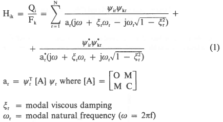
The response function is often written in the form [1]:

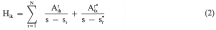
where: and s_r are the residue and root of the expression respectively.

In most practical cases, real modes are assumed which means that the residue consists of the imaginary part only. Therefore substituting:

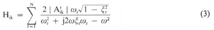
H_ik is the frequency response (deflection) at point i due to unit sinusoidal force at point k.

When ω= 0 then:

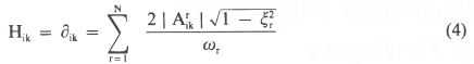
where ∂_ik are the static deflection components of the flexibility matrix [∂].

The information contained in [∂] is sufficient to determine any stiffness required.

In this paper we have used the structure flexibility rather than the structure stiffness defined in the stiffness matrix, nevertheless once [∂] is obtained, the stiffness matrix can be easily found by the relation [2]:

The following conclusions can be made so far:

(1) Structural stiffness can be approximated from FRF at low values of ω.

(2) Structural stiffness information is contained in the FRF and therefore can be determined from the modal parameters

In the next sections it will be shown how these conclusions could be implemented in practice.

 

Determination of Flexibility using an Unbalanced Motor

The method is based on recording vibration signals while an unbalanced variable speed motor is being run up or down. The vibration signal is preferably monitored through a tracking filter into a real time analyser.

Once the motor unbalance (m. e) and the running speed ωis known, it is a simple matter to calculate the stiffness. Assuming that the vibration is recorded in acceleration and at frequencies below resonance, we get

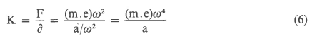
where (me) is the amount of unbalance.

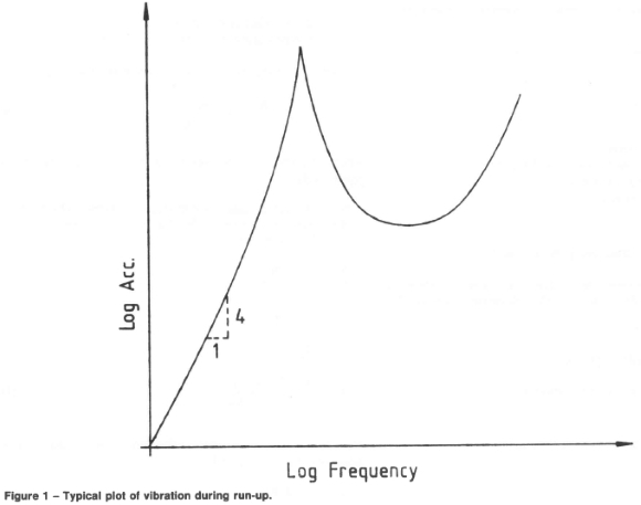
In order to get reliable results one must ensure that the measurements are done in the stiffness control range, where mass and damping effects are negligible. In a logarithmic display that will mean a straight positive slope line free of resonances. A typical plot of vibration during run up is given in figure 1.

 

 

Determination of Flexibility from Modal Parameters

A simple way of obtaining modal parameters is to use an impact technique where a force signal and accelerometer response are recorded simultaneously [3], [4]:

The procedure usually involves some sort of transfer function curve fitting technique for parameter estimation.

A "Gen Rad" analyzer was used in conjunction with "MODAL PLUS" SDRC software, where , ω_τ and ξ_Τ are readily calculated. If the response is obtained in terms of acceleration, equation (4), which is written in terms of deflection, should be changed to:

 

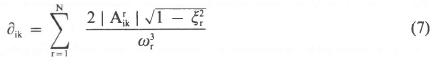
and the flexibility can be derived therefrom.

A typical driving point transfer funtion with its associated parameter estimation is shown in figure 2.

 

Experimental Confirmation

In order to assess the two dynamic methods suggested in this paper a simple experiment was carried out.

A U beam of 100 × 50 × 6 mm was clamped at its ends as illustrated in figure 3.

An unbalanced motor was attached to the middle of the beam in such a way that the excitation could be acting in either the YZ or YX planes and consequently the flexibility in the Y direction could be measured with excitation in two different planes. With the motors attached, the stiffness at the middle of the beam (point A) was measured statically by adding weights and recording deflection. The stiffness was found to be 1,182 MN/m. In addition, it was established that the assembled beam has a resonance around 40 Hz in the vertical direction (Y) and 27 Hz in the horizontal direction (X).

Next the motor was run up while the acceleration signal at point "A" was recorded through a once-per-revolution tracking filter onto a real time portable analyser operating in its peak mode.

The unbalanced force was determined by the expression F = l,2P(Hz) (N). The stiffness was calculated according to equation (6).

The test results are summarised in table 1.

The next stage was to obtain a driving point transfer function at point A using a calibrated hammer and accelerometer. The signals were processed by an analyser to give the required mode parameters.

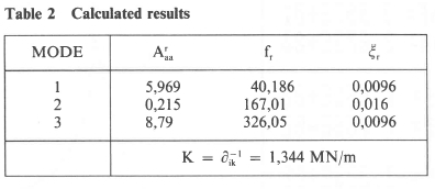
The results of the stiffness calculations using the inverse of equation (7) are summarised in table 2.

 

 

Conclusion

The reasonable agreement is stiffness between static and dynamic flexibility measurement (Static: 1,182 MN/m, Dynamic: 1,127; 1,101 MN/m using unbalanced motor and 1,344 MN/m using modal parameters) suggests the two dynamic methods described here as alternatives to static techniques. Although specialised instrumentation is needed and extra precautions are required, in some cases it could prove to be the only practical way to measure stiffness.

The two dynamic methods have advantages and disadvantages which should be considered for each particular application.

The unbalanced motor is capable of producing higher forces and required relatively simple instrumentation. However, the attachment could be a problem and in some cases can even affect the results.

Problems such as reluctance to drill interface holes in the structure or interface plates not being stiff enough could often be encountered. In these respects the modal parameter method is ideal since it does not require any attachment or interface. However, the instrumentation is more sophisticated and a higher degree of skill is required. For example, the parameters could be estimated only after the operator is convinced of the transfer function quality which can be controlled largely by interchanging the hammer tips.

In the case of the unbalanced motor, recordings should be taken in the stiffness control area. This could cause problems if the structure resonance is low. The motor then has to be run at a very low speed where its force is low.

With the modal parameter method a wider range of frequency is considered. Usually small numbers of modes are required, since the importance of the higher modes diminish rapidly.

Both methods were used successfully on different applications of Escom plant.

 

References

1. CAE International, User Manual for MODAL ANALYSIS 8,0, Structural Dynamics Research Corporation, 1983.

2. Thomson, William T., Theory of vibration with applications, Englewood Cliffs, N J, 1972.

3. Peterson, Edward L., Obtaining good results from an experimental modal survey, Journal of the Society of Environmental Engineers, March 1978.         [ Links ]

4. Schmidtberg, Rupert A., Solving vibration problems using modal analysis, Nicolet Scientific Corporation, 1981.