


Services on Demand
Article
 English (pdf)
 Article in xml format
 Article references
Indicators

Related links
-
 Cited by Google
 -
 Similars in Google
Share

 Permalink
Journal of the Southern African Institute of Mining and Metallurgy
On-line version ISSN 2411-9717
Print version ISSN 2225-6253
J. S. Afr. Inst. Min. Metall. vol.123 n.5 Johannesburg May. 2023
http://dx.doi.org/10.17159/2411-9717/2655/2023
PILLAR DESIGN EDITION
Calibration of the limit equilibrium pillar failure model using physical models
R.P. Els; D.F. Malan
Department of Mining Engineering, University of Pretoria, South Africa
SYNOPSIS
The limit equilibrium model, used in displacement discontinuity codes, is a popular method to simulate pillar failure. This paper investigates the use of physical modelling to calibrate this model. For the experiments, an artificial pillar material was prepared and cubes were poured using the standard 100 mm χ 100 mm civil engineering concrete moulds. The friction angle between the cubes and the platens of the testing machine was varied by using soap and sandpaper. Different modes of failure were observed depending on the friction angle. Of interest is that significant loadshedding was recorded for some specimens which visually remained mostly intact. This highlights the difficulty of classifying pillars as failed or intact in underground stopes where spalling is observed. The laboratory models enabled a more precise calibration of the limit equilibrium model compared to previous attempts. Guidelines to assist with calibration of the model are given in the paper. The limit equilibrium model appears to be a useful approximation of the pillar failure as it could simulate the stress-strain behaviour of the laboratory models.
Keywords: limit equilibrium model, calibration, physical modelling, pillar failure, friction angle.
Introduction
Pillar design for bord-and-pillar layouts is typically done using empirical methods (see Martin and Maybee, 2000; van der Merwe and Madden, 2010). The empirical pillar strength equations are, however, not applicable to all geotechnical areas and there is a risk that the equations are used in mining areas where they are not a good approximation of pillar strength (Malan and Napier, 2011). For example, the weak alteration zones occasionally found in the pillars in the Bushveld Complex reduce the pillar strength and this may lead to mine-wide collapses (Couto and Malan, 2023). A popular alternative is to use numerical modelling, with an appropriate constitutive model, to simulate the rock failure and pillar strength (Sainoki and Mitri, 2017). The failure criteria are typically complex with a large number of parameters to calibrate. These models may therefore not always provide a good prediction of pillar strength and do not always replicate the correct failure mechanism (Malan and Napier, 2011).
A popular approach to simulate pillar failure is to use a limit equilibrium model in a displacement discontinuity code (du Plessis, Malan, and Napier, 2011; Napier and Malan, 2021). This approach is useful as it combines the ability of the displacement discontinuity method to simulate tabular excavations on a mine-wide scale with the limit equilibrium model to simulate on-reef pillar failure. It can simulate the spalling of the pillars, complete pillar failure and the resulting stress transfer to adjacent pillars. This approach is particularly attractive for simulating large-scale bord-and-pillar layouts with irregular pillars (Wessels and Malan, 2023) as well as conventional layouts in the Bushveld Complex with crush pillars (du Plessis, Malan, and Napier, 2011).
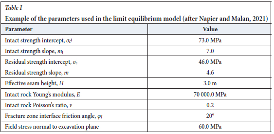
A drawback of the limit equilibrium model is the large number of parameters to calibrate. Table I illustrates the parameters to be calibrated when using this model. Previous attempts to calibrate the model typically involved running simulations with a range of parameter values and comparing the results to underground observations (Napier and Malan, 2021). An improved understanding of the contribution of the various parameters and a calibration strategy is required.
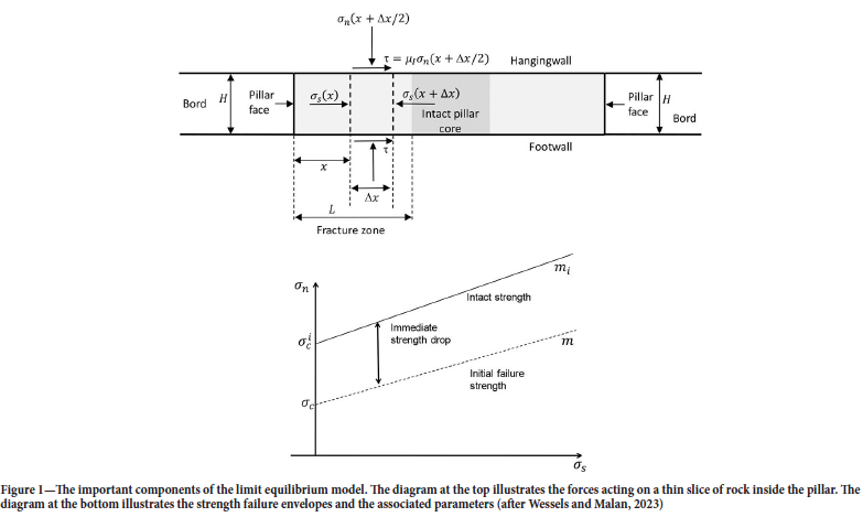
The limit equilibrium model is based on a force equilibrium analysis of a slice of rock in a pillar. The pillar material is bound by frictional parting planes at the hangingwall and footwall contacts (Figure 1). The physical models described in this paper were used to study the effect of this friction angle on pillar strength. In the numerical model, the pillar material can fail and the strength of this material is defined by two envelopes describing the intact strength and the residual strength (Figure 1). These are defined by strength intercept parameters and slope parameters. This basic model can be extended to simulate time-dependent pillar spalling (Wessels and Malan, 2023), but this is not considered in this paper.
An unexplored method to calibrate the parameters shown in Table I is the use of physical models in the laboratory. The use of physical models in rock engineering is described in Napier and Ozbay (1994) and Ozbay, Dede, and Napier (1996). These laboratory models are now seldom used in South Africa, probably owing to the availability of complex numerical modelling codes and the high cost of conducting laboratory experiments. The limit equilibrium model is, however, an excellent example where physical models may be of benefit to better understand the applicability of the numerical model and to devise an improved calibration strategy. This paper describes the initial laboratory experiments that were conducted on model pillars made of an artificial material. One of the objectives of the study was to investigate the effect of friction angle on the hangingwall and footwall 'partings' which delineated the pillar. This was of interest owing to recent modelling that highlighted the detrimental effect of weak layers at these contact planes (Couto and Malan, 2023). The main aim of the experiments was, however, an attempt to validate and calibrate the limit equilibrium model.
Laboratory experiments on artificial pillars
Sample preparation and test methodology
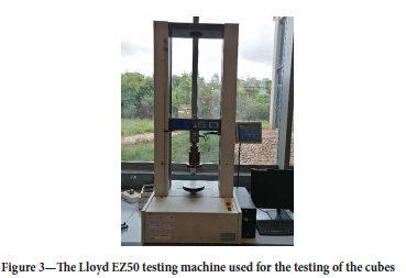
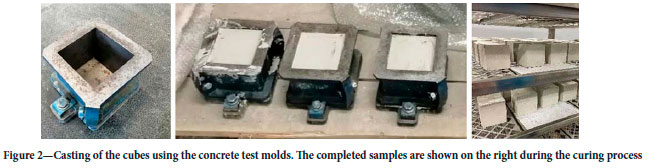
The work was conducted using an artificial material that could be cast. The strength selected for the artificial material was low to ensure that the tests could be easily done in the presses available in the laboratory. The specimens were cast using the standard moulds used for preparing concrete cubes for civil engineering projects (Figure 2). This resulted in specimens with a side length of 100 mm. The casting of the artificial material had a benefit compared to using actual rock as a large number of samples could be cast and tested. The four sides of the cubes inside the moulds were also flat and parallel and two of these opposing sides were used as the contact surfaces with the testing machine. In contrast, achieving flat, parallel surfaces with actual rock material requires expensive and time-consuming sample preparation. Rock samples also typically result in a large variability in strength when conducting laboratory testing. It was hoped that the artificial material would give more consistent results. The drawback of using the standard moulds was that all the 'pillars' tested were cubes with a width to height ratio of unity. The tests were conducted using the 50 kN testing machine in the concrete laboratory of the Engineering 4.0 facility at the University of Pretoria (Figure 3).
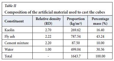
The artificial material used by Jacobsz et al. (2018) and Schoeman (2020) for cave mine modelling in a centrifuge provided the basis for selecting the material for this project. Schoeman (2020) describes a material that was designed to replicate the brittle fracture behaviour of rock, but also to be weak enough to cave. The initial experiments with this material for the pillar project indicated that it was too weak and difficult to handle without breaking the samples. Cement was thus added to the mixture to improve its strength. No sand was added to the mixture. The final composition of the artificial material used by the authors is shown in Table II. Although the mixture contains materials typically associated with geopolymer cement and concrete, the material is not classified as a geopolymer as it contains the cement mixture.
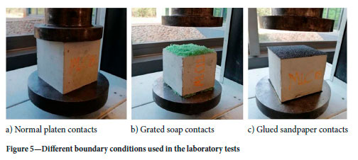
For the experiments, it was planned that all the specimens should have the same composition and dimensions. The only parameter varied was the boundary conditions at the platen contacts to study the effect of the contact friction angle. The 'normal' contact condition was with the steel platen directly applied to the cube. Two other frictional conditions were introduced by using a commercial soap material (to reduce the friction) and sandpaper (to increase the friction) on the contacts between the steel and the cube. The same boundary condition was applied on the top and bottom contact of the cube to simulate the symmetrical attributes of the limit equilibrium model. The soap was grated material and it worked well, but several experiments had to be conducted to refine the sandpaper interface. One attempt was to fold the sandpaper in order to have a sandpaper contact against both the sample and the platen. After trial and error, it was found that glueing the two sides of the sandpaper together gave the most consistent results. For these samples, the contact condition was therefore the rough sandpaper against both the steel platen and the sample, which substantially increased the friction angle.
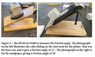
It is known from the literature that the basic friction angles of planar rock surfaces can be determined by means of tilt tests (Alejano et al., 2018). To determine the friction angle of the three types of boundary conditions described above, a simple tilt device was constructed. This is illustrated in Figure 4. A screw mechanism was implemented to ensure that the angle can be gradually increased. The ISRM-suggested method for the tilt test (Alejano et al., 2018) requires that at least five repetitions be performed and the median of the result taken to give the basic friction angle φb = median βi=1,...,5. It was found that the artificial material cubes gave consistent friction angle values throughout and there was no need to determine the median of the five results. The samples against the steel platen gave a friction angle of 21°, the soap contact reduced it to 16°, and the sandpaper increased it to 38°. The set-up of the platen contact conditions in the testing press are depicted in Figure 5.
Test results
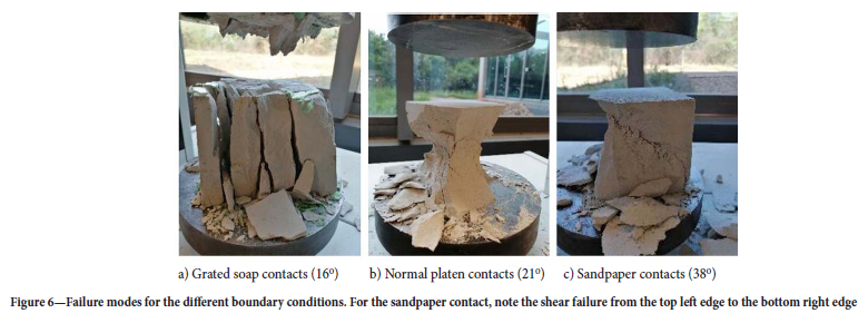
Figure 6 illustrates the typical failure mode of the cubes. The observed mode of failure was consistent for each of the three types of platen boundary conditions and the photographs in the figure are representative of the failure mode for each type. Immediately evident is that the low friction angle specimens underwent axial splitting, while the normal platen conditions with a higher friction angle led to an 'hourglass' failure pattern. These two failure patterns are reminiscent of actual pillar failures observed underground (Malan and Napier, 2011). Further examples of the different types of pillar failures and the effect of a weak layer on pillar strength are given in Wagner (1980) and Esterhuizen and Ellenberger (2007). The sandpaper boundary condition typically led to the formation of an inclined shear between two opposing sides from a top to a bottom corner. These laboratory tests are therefore useful to test the limit equilibrium model as three distinctly different modes of failure are observed. It was initially not clear if the limit equilibrium model is a good approximation for all three cases.
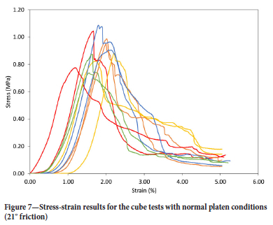
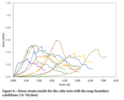
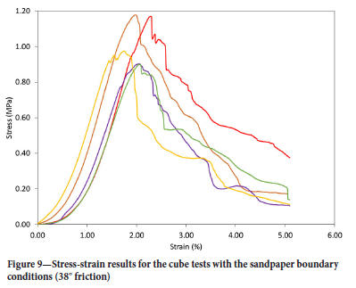
Figures 7 to 9 illustrate the load deformation behaviour of the specimens. The material is weak (peak strength approx. 1 MPa for the cubes with the normal platen conditions) and the post-peak behaviour could be captured by the test equipment. Surprisingly, there is significant variability in the test results, although the specimens were from the same mix. As the tests could not be conducted on the same day, it is not clear if different curing times played a role and this needs to be investigated in future. For all the tests, some 'settling' of the platen on the cube occurred at the beginning of the tests, resulting in the initial flat portions of the curves. This was particularly prominent for the soap contact as the relatively thick layer of soap had to be compacted first. It should be noted that the test conditions may have affected these initial test results and this needs to be explored in future. A spherical seat was not used during the test set-up. The edges of samples in contact with the testing machine were nevertheless considered parallel as two opposing sides of the cubes from inside the moulds were used as the contact surfaces. However, no flatness or parallelism measurements were made. The thickness of the soap layer was controlled by using the same volume of grated soap for each test and efforts were made to spread this soap uniformly across the surface of the specimens to give a constant thickness. This was a crude method and the results should therefore be considered as showing trends rather than providing absolute values. Consideration should be given to how this can be better controlled and measured in future. The initial compaction phase was followed by elastic compression, peak stress, and the post-failure part of the curve. The peak stress for the samples with the soap boundary condition was substantially smaller than for the other two types of tests.
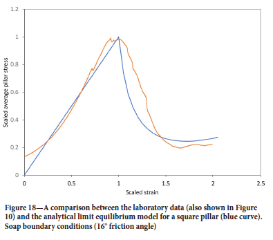
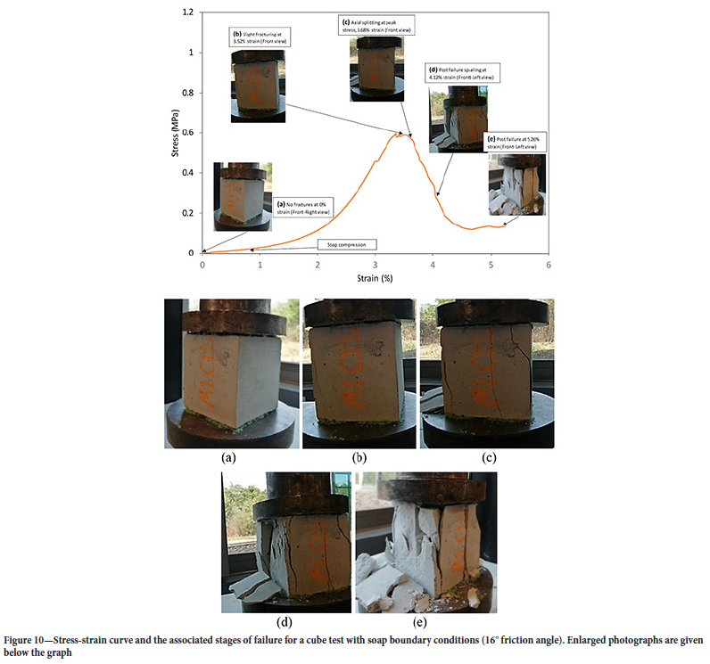
A particular test for each boundary condition was examined in detail and photographs of the state of failure of the 'pillar' were included on the graphs. Figure 10 illustrates a test result with a soap boundary condition. The soap layer needs to be compressed during the early part of the test and therefore significant strain occurs for some samples before the stress starts increasing. In contrast to the test with the other boundary conditions, fracturing is observed only at the peak stress. The strength is also significantly lower. Note that the fracturing recorded for these experiments is based on visual observations only. It is recommended that other techniques, such as acoustic emission monitoring, be used in future to detect the possible earlier onset of fracturing.
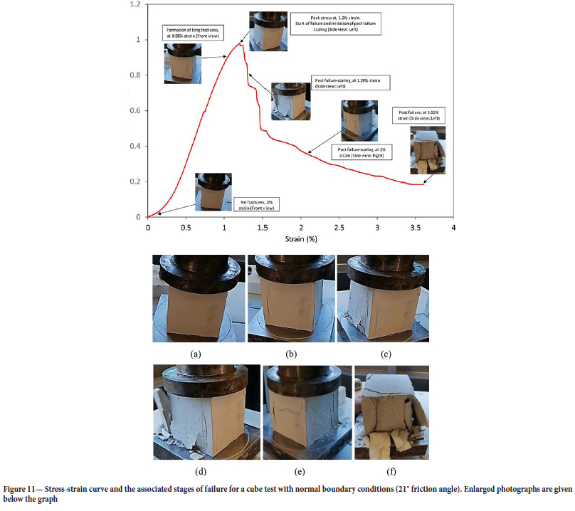
For the normal boundary condition test shown in Figure 11, some fracturing is observed before the peak stress. Significant load-shedding occurs at 2% strain while the sample still appears to be mostly intact. At the end of the test, the core of the pillar still appears to be intact, but significant load-shedding has occurred. This is an important observation in terms of evaluating undergound pillars that are spalling and still appear to be intact. These pillars may in fact be already failed. Failure is evident at the end of the test in the form of an 'hourglass' shape.
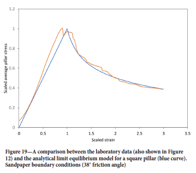
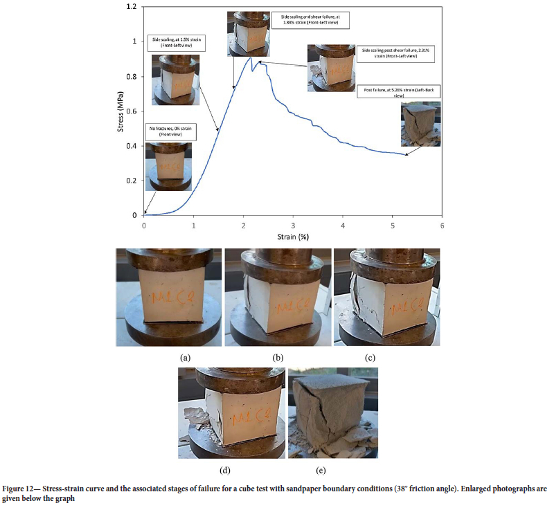
The test with the highest friction angle is shown in Figure 12. The fracturing again starts before the peak strength is achieved. At the end of the test, the inclined fracture running from the top left corner to the bottom right is again visible.
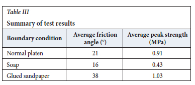
Table III gives a summary of the results with the three friction angles as well as the average peak strengths calculated from the results. Although there is significant variability, there is a trend of increasing peak strength with an increase in friction angle. This is also predicted by the limit equilibrium model modelling and the laboratory testing confirms this attribute of the model. The 38° friction angle did not result in much stronger pillars than the 21° friction angle. This is attributed to the different mechanism of failure (the inclined shear failure).
In the next section we investigate the ability of the limit equilibrium model to simulate these results by considering an analytical model of a square pillar.
An analytical limit equilibrium model of a square pillar
Napier and Malan (2021) derived an analytical solution for the failure of a square pillar, assuming a limit equilibrium model (Figure 13). The detailed derivation of the model will not be repeated here and only a few key equations and additional interpretations are given below. The reader should consult the reference for additional information.
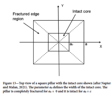
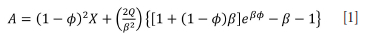
From Figure 13, the width of the square pillar is w=2a. It is assumed that for a limit equilibrium model, the scaled average pillar stress (APS) is expressed by a weighted combination of the average of the stresses in the intact core region and in the surrounding fractured region. Napier and Malan (2021) showed that the scaled APS, A, as a function of the scaled pillar strain, X, can be given by
where the scaled fracture zone length parameter φ is given by
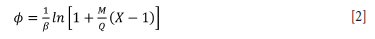
The parameter φ can be considered as a pillar damage variable that ranges from φ = 0 for an intact pillar to φ = 1 for a pillar that is completely fractured. Based on Figure 13, it follows that

In terms of the other scaled parameters, it follows that
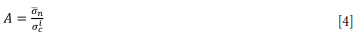
where σ n is the average stress across the pillar (the intact core as well as the fractured edge zone) and σic is the intact uniaxial strength. In terms of the scaled strain,

where εο is the average strain at the point where the pillar stress reaches the postulated intact uniaxial strength σic. The other parameters in Equations [1] and [2] are
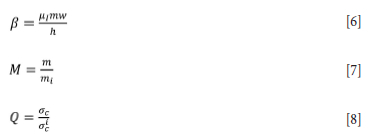
where mi is the slope of the intact limit equilibrium strength envelope, m is the slope of the residual limit equilibrium strength envelope, σic is the intact rock uniaxial strength, and σc is the residual strength after failure (Figure 1 shows an example of these strength envelopes). The parameters w and h are the width and height of the pillar respectively. Furthermore, μ1 = tanφi is the coefficient of friction at the interfaces of the pillar with the hangingwall and footwall and φι is the interface friction angle. These parameters are also given in Table I.
From Equation [1], the scaled APS, A*, for the pillar when the pillar is completely fractured, φ = 1, is given by the simplified equation (Napier and Malan, 2021):

A number of properties of the model are evident from the solution given in Equation [9], and these may be useful when calibrating the model using the laboratory test results. If σc = 0 (or Q = 0), then the residual APS when the pillar is fractured through will be zero. Values of σc > 0 need to be selected. Furthermore, if the friction angle φι tends to zero, (or β -> 0), the residual APS is given by the following solution:
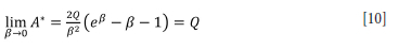
The APS for a friction angle of φι = 0 for a pillar completely fractured will therefore be Q.
To gain insight into the effect of the friction angle, Equation [9] was used to plot A* as a function of friction angle φI. This is illustrated in Figure 14. Note that the y-intercept is the Q value. The graph therefore correctly predicts that  for the parameter values selected.
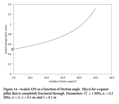
Figure 14 provides a possible method to calibrate the residual strength in the model, σc, from laboratory testing. If 'pillars' can be tested at different interface friction angles, a function fitted to the data can be extrapolated to determine the y-intercept. From this value and the intact strength of the material, the residual strength value can be computed by using Equation [8]. This methodology is illustrated in Figure 15. The same parameter values as Figure 14 were used, but only seven data-points for different friction angles were plotted. The fitted exponential function predicted a y-intercept of 0.45. For the known parameter σic = 1 MPa, the residual strength can be calculated from Equation [8] as 0.45 MPa. This is a reasonable approximation of the correct value of 0.5 MPa.
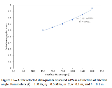
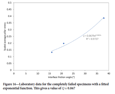
Figure 16 illustrates the actual laboratory data at the different friction angles. The final residual stresses in Figures 10, 11, and 12 (normalized to the intact uniaxial strength, 0.91 MPa) were used for this plot and it is therefore assumed that the laboratory specimens are fractured throughout at these points on the graphs. The data in Figure 16 predicts a y-intercept of 0.067. For the known parameter σic = 0.91 MPa (average of the specimens with a normal platen contact), the residual strength can be calculated from Equation [8] as 0.06 MPa. This was rounded to a value of 0.1 MPa for the additional steps in the calibration process described below. This seems a useful method to calibrate the residual strength parameters, σc, but it is recommended that additional tests be done in future with a greater variety of friction angles to verify this approach.
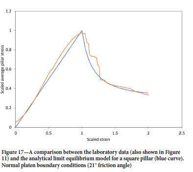
As a first attempt to calibrate the remaining parameters (mi and m), an attempt was made to fit Equation [1] to the stress-strain data presented in Figures 10, 11, and 12. The known and calculated parameter values were used and mi and m fitted. The data from the laboratory tests was scaled similar to the method used for the analytical model (Equations [4] and [5]) to enable a comparison to be made. The origin of the laboratory data was also shifted to the left as the analytical model cannot consider the initial 'compaction' during the early stages of the test. This compaction was particularly prominent for the soap layer. The fitted data is shown in Figures 17, 18, and 19. This was done by trial and error by modifying mi and m to give the best fit. Reasonably good fits between the model and the laboratory data for all three types of test were obtained. The calibrated parameter values are shown in Table IV. It was very encouraging that the experimental curves could be replicated. The only difference between the tests was the friction angle and surprisingly, the curves could be replicated with similar values for the other parameters. The only exception was that a lower value for m was used for the specimen with the highest friction angle (38°). This is not unexpected considering that different failure mechanisms were observed for the three groups of laboratory specimens and the limit equilibrium model is only a simplified approximation.
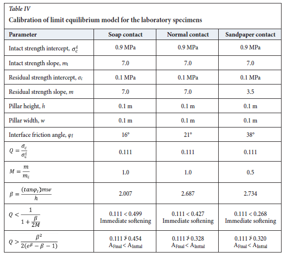
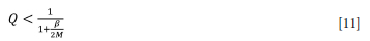
Also, of value for the calibration process is that the limit equilibrium model can predict strain softening or hardening after the onset of failure. According to Napier and Malan (2021), the condition for immediate softening at the onset of failure for a square pillar is
where β, M, and Q are given in Equations [6] to [8]. Furthermore, the constraint that the final pillar stress (AFinal) is greater than the APS at the onset of failure (Ainitial) is given by
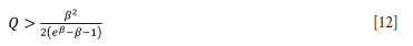
Equations [11] and [12] define whether there is initial softening or hardening of the APS at the onset of failure and the residual hardenend or softened state when the pillar is completely fractured. These values were calculated for the calibrated parameters in Table IV and correctly predict that, for all three cases, there will be immediate softening after failure and the final APS will be less than the APS at which the initial failure occurred. The two conditions given in Equations [11] and [12] are valuable constraints that can assist during model calibration.
Guidelines to assist with calibration of the limit equilibrium model
The steps followed to obtain an improved calibration of the limit equilibrium model can be summarized as follows.
> Laboratory testing to determine the intact rock uniaxial strength. For the experiments in the paper, this was assumed to be the strength of cubes tested using normal conditions on the platens. It needs to be confirmed how well this agrees with the standard ISRM test methodology to determine the uniaxial compressive strength. The effect of other parameters such as humidity and temperature also need to be studied as these may affect the rock material strength in the underground excavations.
> Laboratory testing to determine the shear strength of any weak interfaces present in the pillar. Weak alteration zones in the Bushveld Complex are typically thick clay layers and have a different friction angle in dry and wet conditions (Couto and Malan, 2023). These layers and the infilling need to be carefully tested using a shear box setup and appropriate test methodologies.
> Cube testing of intact pillar material at different friction angles may assist to estimate the residual strength of material when using the limit equilibrium solution for a square pillar as described above. Sample preparation using actual rock will be arduous and varying the friction angle between the sample and the test platens is also a difficult practical problem.
> The very weak material used for the experiments in this study made it easy to obtain the complete stress-strain curves. For actual rock specimens, a stiff testing machine with servo-control may be required.
>The analytical limit equilibrium model presented in Napier and Malan (2021) is a valuable tool for testing cubic samples, and this should be studied in detail to ensure its correct application.
The limit equilibrium is an elegant and relatively simple model, to represent pillar failure in displacement discontinuity boundary element codes. This enables the study of mine-wide geometries where pillar failure is encountered on a large scale. If there are complex pillar failure mechanisms however, such as that caused by major inclined discontinuities traversing the pillars, the limit equilibrium may not be able to simulate the failure behaviour well. Care should also be exercised regarding the presence of weak layers. The limit equilibrium model is a symmetrical model, but pillars are frequently encountered where there is only one weak plane present, at for example the hangingwall contact. Further work is required to extend the model to cater for these asymmetrical pillar geometries. In summary, calibration remains a challenge and a larger number of back-analysis studies will have to be conducted before the model can be used with confidence to predict the pillar strength and layout stability for new mining projects.
Conclusions
The work described in this paper illustrated that laboratory experiments, using an artificial rock material, is a valuable tool to assist with the calibration and validation of complex failure models, such as the limit equilibrium model. Physical experiments to assist with rock engineering studies has been neglected in South Africa in modern times and this capability needs to be rebuilt.
The tests on the artificial pillars confirmed once again that the interfaces between the pillar and hangingwall, and the pillar and footwall, have a significant effect on the pillar strength. For these tests, there was approximately a 60% reduction in average pillar strength (Table II) when the friction angle on the interface decreases from 38° to 16°.
The limit equilibrium model could simulate the reduction in pillar strength for a decrease in friction angle on the interfaces. It also successfully simulated the stress-strain behaviour of the pillars. This work therefore illustrates the value of the model, provided the parameters can be calibrated. A drawback of the current model is that it assumes a symmetrical geometry with weak partings at both the hangingwall and footwall. This could be easily replicated in the laboratory with the artificial pillars, but is rarely encountered in underground stopes where only one weak plane may be present. Further work therefore needs to be done to extend the model to account for asymmetric conditions.
Additional laboratory work using a wider range of friction angles will also be useful to verify the calibration methodology proposed in the paper. It is not easy to find suitable materials to reduce or increase the friction angle on the interface in a stepwise fashion. It was also disappointing that the artificial pillar material still resulted in significant variability in strength for the various samples tested. The reasons for this need to be explored to reduce this variability in future experiments.
Acknowledgements
This work forms part of an MEng study by Ruan Els at the University of Pretoria. The authors would like to thank the Civil Engineering Department of the University of Pretoria for the use of their facility and equipment.
References
Alejanö, L.R., Muralha, J., Ulus AY, R., Lí, C. C., Pérez-Rey I., Karakul, H., Chryssanthakis, P., and Aydan, Ö. 2018. ISRM suggested method for determining the basic friction angle of planar rock surfaces by means of tilt tests. Rock Mechanics and Rock Engineering, vol. 51. pp. 3853-3859. [ Links ]
CouTO, P.M. and Malan, D.F. 2023. A limit equilibrium model to simulate the large-scale pillar collapse at the Everest Platinum Mine. Rock Mechanics and Rock Engineering, vol. 56. pp. 183-197. [ Links ]
Du Plessis, M., Malan, D.F., and Napier, J.A.L. 2011. Evaluation of a limit equilibrium model to simulate crush pillar behaviour. Journal of the Southern African Institute of Mining and Metallurgy, vol. 111. pp. 875-885. [ Links ]
Esterhuizen, G.S. and Ellenberger, J.L. 2007. Effects of weak bands on pillar stability in stone mines: Field observations and numerical model assessment. Proceedings of the 26th International Conference on Ground Control in Mining, Morgantown, W.V. Peng, S.S., Mark. C., and Finfinger, G. (eds). https://www.cdc.gov/niosh/mining/userfiles/works/pdfs/eowbo.pdf [ Links ]
Jacobsz, S., Kearsley, E. P., Cummlng-Potvln, D., and Wesseloo, J. 2018. Modelling cave mining in the geotechnical centrifuge. Physical Modelling in Geotechnics, vol. 2. CRC Press. [ Links ]
Malan, D.F. and Napier, J.A.L. 2011. The design of stable pillars in the Bushveld mines: A problem solved? Journal of the Southern African Institute of Mining and Metallurgy, vol. 111. pp. 821-836. [ Links ]
Martin, C.D. and Maybee, W.G. 2000. The strength of hard-rock pillars. International Journal of Rock Mechanics and Mining Sciences, vol. 37. pp. 1239-1246. [ Links ]
Napier, J.A.L. and Malan, D.F. 2021. A limit equilibrium model of tabular mine pillar failure. Rock Mechanics and Rock Engineering, vol. 54. pp. 71-89. [ Links ]
Napier, J.A.L. and Ozbay, M.U. 1994. The role of physical modelling in the calibration of numerical models. Application of Numerical Modelling in Geotechnical Engineering. Proceedings of the SANGORM Symposium, Pretoria. South African National Institute of Rock Engineering, Johannesburg. [ Links ]
Ozbay, M.U., Dede, T., and Napier, J.A.L. 1996. Physical and numerical modelling of rock fracture. Journal of the South African Institute of Mining and Metallurgy, vol. 96, no. 7. pp. 317-327. [ Links ]
Salnoki, A. and Mitri, H.S. 2017. Numerical investigation into pillar failure induced by time-dependent skin degradation. International Journal of Mining Science and Technology, vol. 27, no. 4. pp. 591-597. [ Links ]
Schoeman, N. 2020. The effect of overburden and horizontal confining stress state on cave mining propagation. MEng dissertation, University of Pretoria. [ Links ]
Van der Merwe, J.N. and Madden, B.J. 2010. Rock Engineering for Underground Coal Mining. 2nd edn. Special Publications Series 8, Southern African Institute of Mining and Metallurgy, Johannesburg. [ Links ]
Wagner, H. 1980. Pillar design in coal mines. Journal of the South African Institute of Mining and Metallurgy, vol. 80. pp. 37-45. [ Links ]
Wessels, D.G. and Malan, D.F. 2023. A limit equilibrium model to simulate time-dependent pillar scaling. Rock Mechanics and Rock Engineering, vol. 56. pp. 3773-3786. [ Links ]
 Correspondence:
D.F. Malan
Email: francois.malan@up.ac.za
Received: 25 Feb. 2023
Revised: 31 May 2023
Accepted: 13 June 2023
Published: May 2023

