PROFESSIONAL TECHNNICAL AND SCIENTIFIC PAPERS

 

Simulation of production processes and associated costs in mining using the Monte Carlo method

 

 

M. Mathey

Visiting Adjunct Professor, Wits Mining Institute, University of the Witwatersrand, Johannesburg, South Africa

Correspondence

 

 

---

SYNOPSIS

The application of the Monte Carlo technique to production planning and everyday economic decisionmaking in mine production management is demonstrated. The logic is detailed using an example of underground production with continuous miners (CMs) and truck haulage. It is argued that availability of equipment and personnel are the predominant variables influencing mine output and productivity and that those availabilities may be well represented by binomial probability distributions. The probabilistic model is implemented in a standard Excel® spreadsheet with Palisade's @Risk add-on to facilitate simulations. Starting from model calibration against data obtained from a mine's annual reports, some general interdependencies of availability, utilization, productivity, and costs of production processes are outlined. Finally, several possible options and their consequences as regards production improvements are explored.

Keywords: simulation, production processes, costs, Monte Carlo method.

---

 

 

Introduction

The Monte Carlo method is typically used to simulate the interaction of input variables within a problem logic, in order to identify possible outcomes and associated probabilities. As such it is frequently used in financial analysis of mining projects. Heuberger (2005) provides a general introduction to risk analysis with the Monte Carlo method.

The method is just as well suited to simulating success, risk, and opportunities in technical production processes. For example, Brzychczy (2018) makes use of stochastic networks combined with Monte Carlo analysis to simulate and optimize the performance of longwall operations in coal mining. Jung, Baek, and Choi (2021) propose a discrete event simulation of production in an underground limestone mine. Upadhyay and Askari-Nasab (2018) likewise suggest a discrete event simulation for a shovel-truck production system in opencast mining. Common to those publications is the 'microscopic' focus on the production process itself, where uncertainty is linked to variables such as equipment travel times, the degree of filling of buckets, and productivity rates in general.

The modelling approach selected in the present paper is 'macroscopic', presuming that production outputs in underground mining are predominantly driven by availabilities of equipment and personnel, once equipment types and number of units as well as section layouts and travel distances are decided. Following this argument, the production process may be divided into a number of independent variables, such as the availability of equipment or workforce, and dependent variables, e.g. equipment staffing ratios and productivity. On each given production shift, those variables 'meet' and result into a specific production output with associated costs. Through simulation one may therefore predict the most likely production outcome for a particular business year or find ways to optimize KPIs such as specific cost of production.

This paper showcases an equipment and personnel availability-based Monte Carlo simulation using underground production with continuous miners (CMs) and truck haulage as an example. The technical process design, logic, and associated costs can be implemented in a standard Excel® spreadsheet application. The generation of random input parameters, as required by the Monte Carlo method, may also be accomplished using standard functions provided in Excel. However, for complex simulations, it is advised to use add-on software such as the commercially available software @Risk by Palisade, which provides extensive modelling features (e.g. random number generators, goal seek analysis by adjusting values of cells, and sensitivity analyses).

The probabilistic Monte Carlo approach demands that the model logic is built around probability distributions of input variables, which are specified by the user. A fundamental argument proposed in this paper is that most aspects of availabilities in mining production processes can be adequately represented by binomial probability distributions, as discussed in the following section.

 

Binomial distribution

The term 'availability' refers to a binary condition of equipment and personnel, which can be either available or unavailable for production on a particular operating shift. It is argued (and later demonstrated in a case study) that if the average availability of personnel and equipment units in a given business year is known from experience or by assumption, then the probability of having a given number of equipment units or personnel available on a random operating shift can be predicted by a binomial probability function.

In its general definition, the density function of the binomial probability distribution is expressed as

 

 

where n is the number of trials, p is the probability of success for each trial, k is the number of successes, and b(k,n,p) is the probability of having exactly k successes out of n trials.

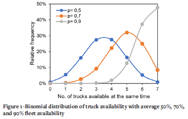
Translated to the context of the production logic proposed here, the binomial density function provides an estimate of the probability of having exactly k equipment units available on a random operating shift from a total fleet of n units with average fleet availability of p.

Example: Assume a mine operating a fleet of n = 7 trucks with average fleet availability of p = 50%, 70%, or 90% on a shift basis. The probability (here expressed as relative frequency) of having exactly k = 0, 1, 2, 3 ... 7 trucks available on a given working shift may then be calculated from the binomial probability function with corresponding curves presented in Figure 1. For example, if the average fleet availability is 70%, one can expect to have exactly five trucks available on 32% of all shifts within a business year.

 

 

More often, however, the production planner requires to know how much equipment from his fleet will at least be available on a given working shift. Assume for instance that the fleet of seven trucks is supposed to serve three CMs for in-section haulage. For the process to work most productively, each CM requires two trucks for haulage. Hence, if all CMs are supposed to work simultaneously, at least six trucks are required to be available at the same time.

According to the binomial distribution for 70% truck availability, one easily calculates the chance of having at least six trucks available on a given shift at only 33% (calculated as the sum of the relative availability of exactly six and seven trucks in Figure 1). This is a very low probability. One could now surmise that the production process is either underequipped and requires additional trucks, or that average truck availability requires major improvement, or both. For proper economic decision-making, however, one must consider that the three CMs themselves will not be always available. The question then is: how often will enough trucks be available for the individual number of available CMs on a given shift?

The problem of group availability - or, in general, matching of two or more independent variables with individual probability distributions at a given point in time - may still be computed using standard spreadsheet applications. Using two separate columns, create equally large binomially distributed random numbers for available CMs in one column and trucks in the other. Then, row-by-row, check how often the criterion is met that at least two trucks are available for each available CM.

The results may be charted as shown in Figure 2. In the given example, a fleet of seven trucks with average 70% availability and a fleet of three CMs with 70% availability can be expected to have 72% group availability. The production situation therefore is already much better than initially estimated based on the availability distribution of the trucks alone. Yet it might still not be good enough.

 

 

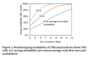
Figure 2 also shows how group availability is expected to improve as more trucks are added to the fleet. The diagram highlights an important point: for all practical purposes, the group availability increases near-linearly in the range of investigation up to a level of approximately 80% group availability. Beyond this level, the binomial distribution curves predict that an increasingly disproportional effort is required to reach as high as 100% group availability, hence questioning the economic meaningfulness of this approach.

So far, we have only considered the results of two independent and binomially distributed variables meeting in the production process. There are, of course, many others. For instance, if a mine requires systematic roof support in conjunction with face advance, the availability of roofbolting equipment may be added to the logic. Likewise, the availability of conveyor belts and processing units might become a focus of investigation as well, and the availability of personnel to operate the available units of equipment .

All relevant factors pertaining to the logic of production with CMs are addressed in the following section.

 

Production modelling

Input variables

A full probabilistic production model must consider all relevant factors pertaining to the production process. To stick with the example of a CM and in-section haulage with trucks, those factors are (compare with Figure 3):

 

 

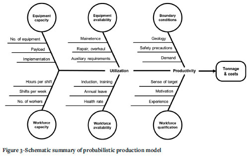
> Production time: Planned production shifts per year and hours per shift.

> Equipment capacity: Number of relevant units of equipment with payload and their respective implementation in the process, e.g. optimum travel distance to the section conveyor and auxiliary (unproductive) work necessary for the process, such as transport from shaft to section, work break, pick change, fresh air extension, equipment relocation etc.

> Equipment availability for groups of equipment, e.g. the fleet of CMs, trucks, and (if applicable) drill rigs or other machines. If the simulation targets optimizing the maintenance strategy, the average fleet availability may be subdivided into further aspects such as frequency of breakdowns, mean time-to-repair, or the share of planned and unplanned maintenance that is expected.

> Boundary conditions: All external impacts on the production system, such as bad ground conditions, additional safety precautions, or limitations pertaining to mineral processing such as demand or availability problems. Such factors can also be implemented (combined with an expected probability of occurrence) in the process logic.

> Workforce capacity: Number of full-time equivalent (FTE) workers allocated to the production team and their distribution across the planned production shifts per day and per week, as well as work hours per shift (i.e. 'hot' or 'cold' seat change).

> Workforce availability: The expected average sick days, share of annual leave, and share of time that is allocated for 'unproductive' (in terms of no tonnage produced) safety induction, training, and the like, resulting in an effective workforce availability for productive work.

> Workforce qualification is another important factor, which can result in higher or lower levels of productivity. For instance, a mine operating with well-rehearsed teams or piecework reimbursement contracts may see higher productivities, and others which operate with a large proportion of unskilled miners or contract workers may perhaps see lower productivities. All such influences, if relevant to the analysis, may be implemented accordingly.

The idea of the Monte Carlo simulation is to simulate a large variety of probable constellations of the above-listed variables per shift and to process the variables using the individual production logic to result in tonnage output, which is then extrapolated to a full business year.

For each simulated shift the production logic needs to check the number of available units of equipment (with minimum staffing requirements) against the available personnel. This step determines if any bottlenecks exist on the technical side (see truck vs. CM problem) and how much equipment can be effectively utilized for production.

In a more refined production logic, the key decision of utilization must also consider all options available to the team leader, such as: is it possible to substitute a missing truck by using an available LHD or another load-carrying unit and by how much will this reduce the overall process capacity? Are there further boundary conditions related to the mineral processing side which prohibit full utilization? How do I distribute the available personnel most effectively across the equipment to result in maximum tonnage?

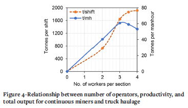
In fact, the problem of utilization is one of optimal resource allocation under varying boundary conditions and directly affects the productivity (i.e. the specific tonnage output) of the simulated shift. This fact must already be accounted for in the process design and workforce planning. For example, one can easily imagine that allocating an increasing number of employees to a CM section may result in an increase in tonnage output, at least up to a certain level. However, the specific labour productivity (tons per man-hour) will decrease from some point.

Figure 4 shows such a staffing-productivity relationship for a typical CM section. The labour productivity curve peaks at around 3.2 workers per section (that is, three workers to operate the CM and two trucks plus 0.2 worker to compensate for work breaks, during which, if not accounted for, the process would either stop entirely or at least decrease in productivity). If more personnel are allocated to the section, auxiliary work such as a pick change or extension of layflats for fresh air supply may be completed more quickly and hence contribute to more production time per shift and tonnage output. However, the tonnage output cannot increase in proportion to the additional man-hours and hence labour productivity in terms of tons per man-hour declines.

 

 

Such information is vital to the quality of a production model and, if available, the respective relationships can be easily tabulated and implemented in the Excel-based simulation.

More variables may be added as required as outlined above. For example, if there is a 20% probability that tough geological conditions reduce a shift's output by, say, 10% (e.g. because a CM's cutting speed is limited by the strength of rock), then this can be simulated accordingly. However, as the number of variables in the model increases, so does the level of complexity by a disproportional amount and care must be taken that the relationships and causalities of the production process are still programmed in the correct way. It is therefore advisable to set out a clear scope of analysis and include only a minimum number of parameters identified as truly essential to the problem.

Simplified simulation procedure

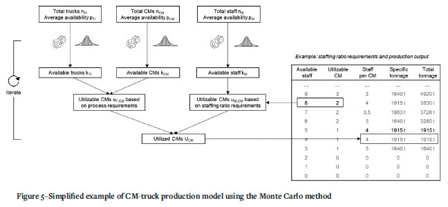
In a simplified CM-truck production system that is free from limiting boundary conditions (e.g. tonnage demand limitations, limitations from auxiliary processes, geological limitations etc.) the sequence of the Monte Carlo process simulation is as follows (see also Figure 5):

Step 1: For both equipment categories (trucks and CMs), define the total number of units n_CM, n_Tr with respective average availabilities p_CM and p_Tr to create the binomial availability distribution for both categories.

Step 2: For the workforce, define the total number of staff n_st with average availability p_st.

Step 3: Define the desired staffing ratio between available personnel and available CM-truck systems with corresponding productivities (such as suggested in Figure 4) in a table.

Step 4: For a random working shift within a business year, generate a random number of available items of equipment k_CM, k_Tr and random number of available staff k_st from the binomial probability distributions defined in steps 1 and 2.

Step 5: Compare CM vs truck availability from step 4 and calculate the technically utilizable number of CMs u_TCM based on process requirement, e.g. as the minimum number of trucks that need to be available for one CM to be utilizable.

Step 6: Calculate the number of CMs u_ST,CM that can possibly be utilized based on the number of available personnel and the table defined in step 3.

Step 7: Select the number of items of equipment to be utilized on shift UCM, which equals the minimum value of either u_T,CM or u_StCM, and the corresponding staffing ratio per utilized CM.

Step 8: Calculate tonnage output and tons per man-hour on shift from the table (step 3).

Step 9: Iterate through steps 4-7 repeatedly, preferably >1o 000 times for fill representative sample (Monte Carlo method).

This simulation procedure will result in a variety of production outputs per shift which need to be multiplied with the number of planned operating shifts per year to derive annual results.

 

Case study

The outlined Monte Carlo simulation logic is applied to a real mining situation to showcase how such a model may be calibrated, what the interdependencies of process parameters with effect on tonnage output and costs are, and how the model can be applied to find ways to optimize production.

The selected case study is an underground room-and-pillar mine in a soft rock environment, which produces about 4 Mt ROM per annum from both conventional drill-and-blast-sections and CM sections (the latter being the focus of the case study). The mine operates three CMs with a fleet of seven trucks for in-section haulage, as discussed before. A full set of data (technical data, shift reports, KPI reports, and others) from a given business year is available for evaluation and serves as a basis for model calibration. The productivity diagram in Figure 4 has been derived from this empirical data and is implemented in the model.

Equipment availability

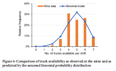
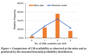
The first step in applying the model is to check if the underlying assumption of binomial probability distributions for equipment availability is correct. In the particular business year, the average availability of the truck fleet was 70.4% and the related histogram of truck availability as derived from shift reports is plotted in Figure 6, together with a binomial model of truck availability using the identical input data (n = 7, p = 0.7). The same comparison is made for the fleet of CMs in Figure 7, where n = 3, p = 0.61 as obtained from the mine's reports. One observes an overall acceptable match between the assumed binomial distributions and reality.

 

 

 

 

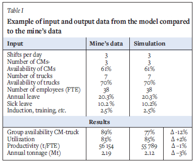
The next step is to implement all remaining input variables based on the actual mine data and the process logic as described above, and to test the model. Some key input factors and model results are summarized in Table I.

 

 

Group availability

A group availability of 89% was established from the mine's reports, compared to only 77% predicted by the model, as shown in Table I. The positive discrepancy of 12% is appreciable and may be due to two reasons. The first is on the side of theory: obviously, the fitted binomial distributions of truck and CM availabilities match the real data well, as seen in Figures 6 and 7, but there is no 100% fit. Hence, through error propagation, a combination of the two distributions will produce (possibly larger) mismatches. The second reason is on the practical side: the mine had successfully prioritized its maintenance efforts to make sure that (as often as possible) enough trucks were available at the time they were required for a given number of CMs. That is, through correct resource allocation the mine was able to 'beat' the average statistic. Such effects do not question the principle of modelling but must be borne in mind when interpreting and making decisions based on models.

The mine's report also revealed that if a truck was missing in the production chain, it could frequently be substituted by an LHD with only slightly smaller payload from the adjacent drill-and-blast sections. Consequently, this improvement was introduced as a general rule in the production simulation (i.e. every missing truck can be substituted by an LHD), so that the lower CM-truck group availability does not influence the predicted utilization, productivity, and tonnage output too much, as can be seen in the following section.

Utilization, productivity and tonnage output

Next, one introduces the variable of workforce availability, allowing for the 33% of time that workers were evidently not available for utilization of available equipment due to annual leave, training, or sickness. The model computes an equipment utilization of 85% on a shift basis, which compares favourably with the 83% utilization in the business year. Also, the simulated annual tonnage and the related tons per employee stand the reality check very well, as shown in Table I.

Note that the results are probabilistic. Figure 8 provides a detailed plot of the simulated annual tonnage output from the mine. The bar chart features three main peaks:

 

 

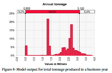
> The first peak is at zero tonnage and indicates that at around 6% of the annual production time, there will be zero tonnage output. This point corresponds to the binomial model for CMs (Figure 7) which predicts a 6% chance that none of the CMs will be available during the business year.

> The next peak occurs at around 1.3-1.5 Mt and represents the productivity during all those situations in which only one CM will be available, scaled up for a whole business year.

> Finally, a third peak at around 2.7 Mt, which is accompanied by a larger scatter to its left and right. This interval represents all those situations in which 2-3 CMs are available for production in a range of sub-optimal (i.e. insufficient number of workers or trucks available) to optimal combinations. Again, the productivity of those situations is scaled up for the whole business year.

Note that, due to the scaling logic, the most probable production output is determined from the average simulation result, i.e. 2.12 Mt in this case study.

 

Analysis of production and associated costs

Based on the calibrated model some fundamental relationships and principles of the production process can be examined. For instance, consider the relationship between average CM availability and planned utilization. In the given example, three CMs operating in a three-shift-per-day system allow for utilization of up to nine machine-shifts per day (see Figure 9).

 

 

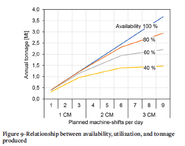
Evidently, there can be a straight-line relationship between planned-utilization and annual output only if the CM availability was 100%. For all availabilities < 100%, output only increases regressively with an increase of planned production shifts.

Consider the curve for 60% average CM availability: the chance of having at least one CM available on each shift is relatively large (93%, calculated as the cumulative probability of having exactly 1, 2, and 3 CMs available using the binomial distribution with k = 1, 2, 3 respectively; n = 3, p = 0.6 as described in the section 'Binomial distribution'), so that the gradient of output from the first three planned machine-shifts per day is relatively steep. The next 4-6 planned machine-shifts per day require that at least one additional CM is available, the chance of which is already less (65%). Finally, machine-shifts 7-9 require that three CMs are available simultaneously on one to three shifts per day, the chance of which is the lowest (22%).

At the same time, each additional planned machine-shift per day requires that a proportional number of workers is permanently employed (since one can rarely foresee when a machine will be available or not), whose specific output in terms of tonnage per employee reduces since the absolute tonnage output increases at a slower rate. Equipment availability and workforce productivity are obviously interlinked.

Next, a full set of production costs may be added to the model. From an accounting point of view, there will be fixed costs, such as annual depreciation of equipment and cost of labour for a given number of planned utilization shifts. Other costs are variable, i.e. in some ways proportional to operating hours and tonnage output, such as energy and consumables. Some mines may also find that the cost of maintenance is - at least from a long-term average perspective - proportional to the operating hours of equipment and therefore to tonnage.

The above-named cost categories have been implemented in the model assuming realistic values. Figure 10 shows the computed relationship between annual output and expected specific cost of production. At first, all cost curves show the same regressively decreasing trend. If this trend was to continue for very large production outputs, the fixed part of the cost would become negligibly small and the overall specific costs would tend towards the value of the variable costs. Clearly, this cannot be the case in a real production process, as marginal costs come into effect as well: from a certain point onwards, the cost curves reverse, as every additional tonnage output requires a disproportional amount of effort.

 

 

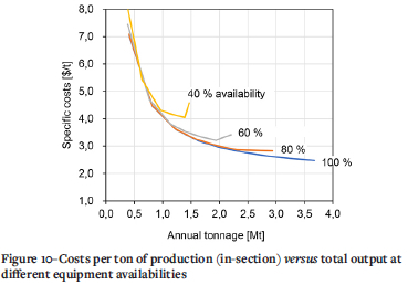
In the example shown in Figure 10 this marginal effect is only due to the inefficient low availability compared to high staffing. However, other factors such as extending production to overtime (surcharge), adding additional equipment to ensure higher output, or increasing the staffing ratio towards a production maximum such as shown in Figure 4 may work to the same effect.

The relationship in Figure 10 clearly indicates that, depending on the level of equipment availability, there might be an optimal point of production in terms of minimum specific costs. However, there might be at least two good reasons why production should perhaps be extended beyond this point:

> Underground mines are typically associated with a very large portion of fixed costs (e.g. shafts, conveyors, processing units), so that a sub-optimal cost increase within the production sections may become irrelevantly small in overall terms.

> Sub-optimal costs of production may be over-compensated by exceptionally good selling prices.

Nevertheless, if the company's focus is on optimizing internal costs of production, or at least to increase production while incurring minimum additional costs, the Monte Carlo simulation can assist in negotiating the various possible approaches. Some examples are provided in the following section.

 

Optimization

Returning to the case study and the calibrated model, one may now ask several questions as to possible production improvements. The iterative process of querying various parameter combinations is greatly facilitated in @Risk by using the built-in simulation and optimization tool. Some examples:

> How does the addition of an eighth truck to the fleet enhance the annual production, assuming the average availability of the fleet does not change? Answer: An extra 30 000 t of production. Note that this result must be interpreted with care, since the model makes use of the simplified rule that every missing truck can be substituted with an LHD. If this is not the case, the benefit from purchasing an eighth truck is larger than 30 000 t.

> Alternatively, what must the average availability of the seven-truck fleet be to achieve the same increase of 30 000 t/a in perhaps a cheaper way? Answer: 79.6% (a 7.6% increase).

These two alternatives must be negotiated from a cost and reliability point of view. On the one hand, the purchase of an additional truck provides a certain reliability but comes at the disadvantage of additional costs. On the other hand, attempting to improve the availability of the existing fleet may come - through optimization of internal processes - at lesser cost, but may be more difficult to achieve. Other examples:

> How does an increase of 5% in equipment availability for both trucks and CMs compare to a 5% improvement in the health of the workforce (i.e. personnel availability)? Answer: An increase of approximately 160 000 t/a versus 73 000 t/a.

This comparison demonstrates that for the given case study, equipment availability is a more effectful lever than worforce availability. The more so as workforce health is to a large extent dependent on aspects outside of the employer's realm of influence. Final example:

> At the given average equipment and workforce availability, what is the optimal number of workers employed within a business year, in terms of maximum tons mined per employee?

Answer Reduce planned utilization to two CMs per shift at 3.2 workers per section, totalling about 65 000 t per employee and year (a 16% increase). Note that the mine's annual output from CM sections will reduce to 1.6 Mt only (a drop of -26%).

The examples showcase the strength of the model in providing quick guidance through the economic decision-making process.

 

Conclusion

Successful mining is strongly dependent on the availabilities of equipment and workforce. Since those availabilities are highly variable throughout a business year, resulting in wide ranges of favourable to unfavourable conditions for production output and related productivity, a probabilistic approach to production modelling that makes use of the Monte Carlo method has been proposed.

A fundamental finding in this paper is that availabilities can be modelled with binomial probability distributions and input parameters as obtainable from a mine's report (or from estimation). It has been argued that those binomial distributions, together with a specific process logic, can be implemented into standard spreadsheet application to create a production model which conclusively explains technical and economical relationships of production, such as the occurrence of marginal costs.

The model has been applied to a case study of a selected underground mine, where it was able to accurately predict the mine's performance in terms of tonnages and productivities in a given business year. Against that background, various relationships between the number of units of equipment, equipment availabilities, and number of staff with respective availabilities have been explored to improve the mine's production on a system level.

It is tempting to simulate 'ultimate' questions that pertain to production optimization, e.g. how a mine can produce a maximum tonnage at minimum unit cost, or at least a maximum tonnage with the given resources at hand. The model will indeed produce several outputs with suitable suggestions.

However, it must be borne in mind that the variable nature of equipment and personnel availabilities, as discussed in this paper, is testament to the fact that it takes much effort to manage, allocate, and develop the resources at hand and to lead production towards its goals. In this context, the presented Monte Carlo production model is best understood as a tool which assists mine planners and management in negotiating different strategic decisions. For the strategic decision to become a success, continuous improvement and controlling is required.

 

References

Brzychczy, E. 2018. Probabilistic modeling of mining production in an underground coal mine. Proceedings ofthe International Conference of Intelligent Systems in Production Engineering and Maintenance. Advances in Intelligent Systems and Computing, vol. 835. https://doi.org/10.1007/978-3-319-97490-362        [ Links ]

Heüberger, R. 2005. Risk analysis in the mining industry. Journal of the South African Institute of Mining and Metallurgy, vol. 105, no. 2. pp. 75-79        [ Links ]

Jung, D., Baek, J., and Choi, Y. 2021. Stochastic predictions of ore production in an underground limestone mine using different probability density functions: A comparative study using big data from ICT System. Applied Sciences, vol. 11, no. 9. 4301 p. https://doi.org/10.3390/app11094301        [ Links ]

Upadhyay, S.P. and Askari-Nasab, H. 2018. Simulation and optimization approach for uncertainty-based short-term planning in open pit mines. International Journal of Mining Science and Technology, vol. 28. pp. 153-66.         [ Links ]

 

 

Correspondence:
M. Mathey
Email: Markus_Mathey@web.de

Received: 13 Apr. 2022
Revised: 18 Aug. 2022
Accepted: 17 Oct. 2022
Published: December 20223