PROFESSIONAL TECHINICAL AND SCIENTIFIC PAPERS
http://dx.doi.org/10.17159/2411-9717/2024/2022

 

Defining optimal drill-hole spacing: A novel integrated analysis from exploration to ore control

 

 

B.C. Afonseca^I; V. Miguel-Silva^II

^IAngloGolcl Ashanti - Sabará, Minas Gerais, Brazil. https://orcid.org/0000-0001-9567-4937
^IIVale - Nova Lima, Minas Gerais, Brazil. https://orcid.org/0000-0001-7502-9543

Correspondence

 

 

---

SYNOPSIS

Drill-hole spacing analysis (DHSA) and optimization are becoming commonplace for uncertainty assessment and management in the mining industry. However, there is no standardized DHSA workflow, and the outputs of certain methodologies are not interchangeable. We group available simulation-based DHSA methods according to their accounted uncertainty into (i) raw uncertainty, assessed by drawing realizations from synthetic data-sets with the drilling spacings to be tested; and (ii) model uncertainty, in which these synthetic data-sets are used to assess the variation between the estimated model and the (unknown) actual value. DHSA workflows available in the literature ignore the differences between both types of uncertainty. Commonly, the DHSA algorithm is chosen without a detailed analysis of its uncertainty output, which may lead to misleading results and suboptimal decisions. While available solutions are based only on assessing raw or model uncertainty, the proposed approach simultaneously analyses both and their relationship for models at different stages of the mine. The integrated analysis results deliver more information to support decision-making than available methods. Principles, practical considerations, and discussions of the advantages of the proposed integrated analysis are presented. The approach is applied to a real gold deposit to illustrate its use.

Keywords: drill-hole spacing analysis, conditional simulation, ordinary kriging, uniform conditioning, estimation error.

---

 

 

Introduction

Drill-hole spacing analysis (DHSA) is a set of geostatistical techniques applied to assess the associations among the uncertainty of the estimates, drilling spacing, and data availability. In this sense, the Joint Ore Reserves Committee (JORC, 2012) states that the reporting of Mineral Resources should be supported by significant geological information for all classifications of Inferred, Indicated, and Measured Mineral Resources. The reports must include evidence of the sampling methods and the appropriateness of data spacing to the mineral deposit's geological, physical, chemical, and mineralogical features. DHSA may provide important decision drivers from initial exploration to production models. Its outcomes may also be analysed from an optimization perspective, where we look for the optimal drill-hole spacing (the decision variable) to define an objective function to be optimized, such as a minimum misclassification, maximization of resource conversion, or the best balance between the sampling costs and operational losses caused by under-sampling (Li et al., 2004; Boucher, Dimitrakopoulos, and Vargas-Guzman, 2005; Koppe et al., 2011; Martínez-Vargas, 2017). DHSA tends to be understood as applicable exclusively for diamond or rotary drill-holes. However, these geostatistical techniques may be used to assess the spacing of any type of samples, such as production blast-holes or underground channel sampling. Hereafter, we use drilling and sampling spacing interchangeably to refer to the spacing of the type of data under analysis.

There is no standardized workflow for DHSA, but we may generalize the state-of-the-art and most widely used solutions into kriging- and simulation-based methods. Compared to kriging methods, the simulation-based algorithms demand considerably more computational and technical resources for running, processing, and checking all drawn realizations (Verly, Postolski, and Parker, 2014). DHSA, based on simulation algorithms, provides access to the probability distribution and properly considers the local

variability, proportional, and support effects. We consider that the additional effort required by simulation algorithms is justified due to the risk of losses from suboptimal sampling strategies. Verly, Postolski, and Parker (2014) state that when the risk assessment requirements are not so complex or when the time to complete a simulation is lacking, DSHA involving kriging variance calculations can be useful.

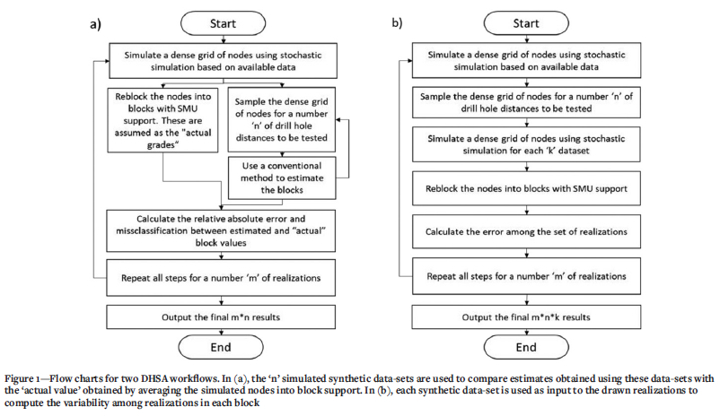
We distinguish the simulated-based methods available in the literature into model uncertainty and raw uncertainty. This distinction is based on the workflow employed to measure the uncertainty in each case. In both algorithms, a set of synthetic data-sets corresponding to the drilling spacings to be tested is drawn by geostatistical simulation. However, on the model-uncertainty workflows (Figure 1a), these synthetic data-sets are input to a chosen kriging estimator. The local accuracy is assessed through the variation between the estimated model and the (unknown) actual value. In the second workflow (Figure 1b), named raw uncertainty, realizations are drawn from each synthetic data-set. The assessment of global accuracy of properties, such as tonnage versus grade relationship, is prioritized at the expense of local accuracy.

Both workflows presented in Figure 1 are widely discussed in the literature. However, the implications, distinctions, and relationship of their output uncertainty is an overlooked subject. The difference between the introduced raw and model uncertainties is directly connected to global and local accuracy concepts. The method in Figure 1a is affected by the fact that kriging methods, by definition, cannot be simultaneously conditionally unbiased and globally accurate. If a resource model accurately predicts the tonnages and grades available for selection at the time of mining, then the block grade estimates are conditionally biased. This is the kriging oxymoron discussed by Isaaks (2005). Based on this concept, DHSA should not be applied without considering the objective function to be optimized, the geostatistical methods, and an adequate definition of its parameters.

The novelty of the presented workflow lies in the fact that DHSA studies should always consider the interdependence between the function being minimized, the method employed for modelling the uncertainty, and the purpose of the models from which decisions are made, from the required accuracy of global grade-tonnage relationship at exploration stages to the local accuracy required to classify mineable blocks of production models. This is especially true when global and local accuracies are compared (Journel and Huijbregts, 1978; Isaaks, 2005). We propose a novel solution in which raw and model uncertainty support an integrated analysis where each type of uncertainty complements the other. Their relationship is fundamental for supporting decision-making. The available algorithms are adapted to generate comparable and interchangeable outputs (Figure 1).

We address this subject as follows. We first distinguish the objective functions for short- or long-term models and their purposes. We analyse the singularities of both reviewed groups of DHSA methods and the objective function optimization, and discuss specifics. Next, we establish a distinction between the raw and model uncertainties. The approach formulated herein is then outlined. We argue that their results are not equivalent, directly comparable, or conceptually similar in some instances. Subsequently, the proposed approach is tested for a real gold deposit, where the raw and model uncertainties are merged for a unique risk assessment. This is followed by a discussion and conclusions.

Literature review: Raw and model uncertainty approaches

Various authors have presented optimization methods for drilling spacing to reduce the uncertainty of the transfer functions of interest. Geostatistical simulation methods are increasingly applied for DHSA because these stochastic methods are recognized tools for quantifying the spatial distribution of uncertainty. The scope of this literature review is not to present details for geostatistical simulation (Deutsch and Journel, 1998; Goovaerts, 1997) but to discuss the differences between the most popular DHSA approaches based on simulation.

We may separate these methods into two groups based on their output uncertainties.

> The raw uncertainty approach (Figure 1b) accurately assesses the global risk attached to a random function (RF) spatial distribution. Synthetic data-sets representing the drilling spacings to be tested are simulated. Realizations are drawn from each data-set. The probability distribution of transfer functions, such as operational costs, net present value, or other economic and engineering parameters can, therefore, be calculated. It is generally assessed by Gaussian methods, maximum entropy methods that provide the most 'disorganized' spatial arrangement possible for a given RF. The reproduction of the RF parameters is prioritized at the expense of local accuracy (Goovaerts, 1997). Here, equiprobable realizations are simply a means to represent the uncertainty, and thus it is recommended to submit all realizations through the transfer function to achieve a full distribution of responses.

> The model uncertainty approach (Figure 1a) uses synthetic data-sets to assess the local accuracy. It better predicts the local uncertainty found in short-term and production models, such as the variation between the estimated model and the (unknown) actual value, or the expectation to classify a block as ore or waste correctly. Kriging is a linear algorithm based on the minimization of the error variance to provide accurate local estimates (Matheron, 1963). Therefore, the actual deviation between model estimates and the true value is expected to be lower than the dispersion assessed by simulation algorithms, here classified as raw uncertainty. The model uncertainty also considers the unavoidable smoothing effect and its related conditional bias. The expected value of the true grade based on the estimates is not equal to the estimated value, and generally underestimates high values and overestimates low values (Journel and Huijbregts, 1978).

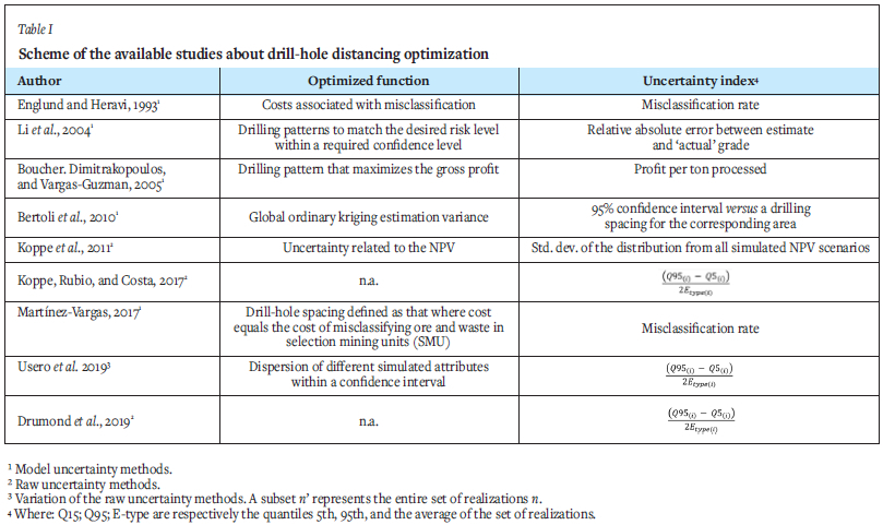
Table I summarizes references in the literature for the approaches defined herein.

One concern associated with both simulation-based groups is their excessive computational requirements. Some authors have suggested the use of scenario reduction, where the objective function would be analysed from a subset m' sampled from m based on similarity or dissimilarity conditions (Armstrong et al., 2013; Okada et al., 2019; Usero, Misk, and Saldanha, 2019). The use of scenario reduction, however, is a disputed subject. The problem to be optimized is key for correctly managing multiple realizations. In general, the full set of realizations should be used for objective functions, such as plan optimization, ultimate pit limits, net present value, or expected profit (Deutsch, 2017). There is no right or wrong realization, as it is impossible to state that one represents the reality better than the others. Incorrect or suboptimal decisions could be made if too few realizations are considered. However, optimization of the drilling spacing for linear objective functions, such as the average estimation error or misclassification rate, can be conducted with fewer realizations. The specific location of high or low variability areas within the simulated domain is not critical. The variability at specific locations averages out globally over multiple realizations, and any of these realizations reflect the overall variability required by DHSA studies.

It is worth emphasizing that the methods discussed here are exclusive for grade uncertainty. No information involving the uncertainty of the geological boundaries of each geological domain is provided by the methods. However, adaptations can capture the joint uncertainty of grade and geological features.

Define the variables and outline the optimization problem

No sampling spacing is optimal by itself. When performing DHSA studies, the drilling spacing is tested against the variable to be optimized, such as the miscalculation rate, resource conversion, or expected profit. The best spacings differ for those different variables. Typical applications for DHSA are as follows.

> Mineral Resource: The DHSA is applied to find the most efficient spacing that supports the resource categories according to confidence levels of the estimates over a large production area. A very frequent practice in the mining industry states that the available information should be enough to support the grade and tonnage prediction within a ±15% accuracy at a 90% confidence interval over a quarterly or monthly production increment for a measured class. The annual production accuracy should be within ±15% at a 90% confidence interval for Indicated Resources. Thus, the DHSA quantifies the investment required for resource conversion or categorization.

> Grade control/production models: The main purpose of grade control models is to provide local precision for the selection of ore and waste. These models provide the last opportunity during mining operations to ensure that the material is correctly assigned to the stockpile or waste dump, which reduces the number of misclassified blocks. The DHSA for grade control is commonly used to evaluate whether a denser drill-hole campaign reduces the block misclassification, the cost of which is, on average, higher than the cost of acquiring new data.

Next, we discuss relevant elements to be considered when performing optimization studies.

The scale of the decisions to be made

Fitting the model scale to the function to be optimized is particularly relevant for DHSA studies. The 'scale of the decision' term addresses the appropriate volume or area relevant for a decision to be made. For instance, in the early project stages, the global grade-tonnage relationship may be much more valuable information for decision-making than the grade accuracy at the mining support. In contrast, assessing the local accuracy, such as the local uncertainty of each estimated block, becomes especially relevant for mining selectivity decisions.

From a geostatistical perspective, the estimation must consider the average distancing of the available data. A widely used rule of thumb states that the block size should vary between 1/4 and 1/2 of the data spacing. This proposition arises from the relationship between the block support, estimation error, and internal block variance. Considering a stationary domain G, the 'smoothing relation' (Equation [1]) explains how the average kriging variance (¾) and dispersion of the estimated block (v) distribution (Df) are negatively related (Journel and Huijbregts 1978):

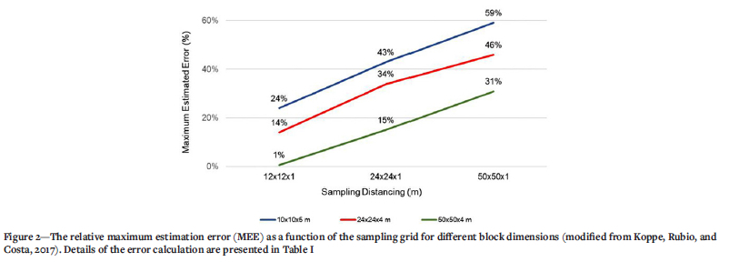
We observe that large blocks are likely to be close to the actual true grade, while very small blocks result in over-smoothed estimates due to the higher estimation variances. Figure 2 shows the influence of the block dimension on the maximum estimated error. Note that the 24 χ 24 χ 4 m block model using 12 χ 12 χ 1 m spaced drill-holes shows uncertainties similar to the 50 χ 50 χ 4 m block model using 24 χ 24 χ 1 m spaced data.

The geostatistical criterion for defining the block size to be used during DHSA leads to a problem in which the block size impacts the drill-hole spacing definition, and vice-versa. Therefore, this paper considers the smallest scale for a decision in mining. It is called a selective mining unit (SMU) size, and production volumes as constant parameters are defined by operational constraints and not as variables to be optimized. An SMU is defined as the minimum volume that allows ore-waste selectivity, which is a function of the mining method and technological conditions.

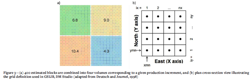
While local accuracy is commonly measured block by block, the global accuracy for resource classification is generally computed for a panel representing a given monthly, quarterly, or annual production increment (Figure 3a). An uncomplicated scheme is often used when a mining plan is not available. Grids commonly employed by commercial mining software packages are sorted out by their x, y, and z coordinates, and then their masses are summed until a desired production increment volume is reached (Figure 3b). Constraints may be applied to mimic realistic operational shapes.

The following section discusses the applicability of raw and model uncertainties from the perspective of different uncertainty indicators, functions to be minimized, and methodologies available in the literature.

 

Proposed methodology

The reviewed DHSA methods focus on setting the relationship between the drill-hole spacing and a specific uncertainty index considering a single model purpose, such as the required local accuracy of production models, or the global accuracy for a resource model. Therefore, DHSA does not connect the optimal drill-hole spacing for an exploratory model with the infill campaign to be drilled in the future. This relationship is not fully captured by the methods available in the literature and no optimal decision can be made without considering an integrated DHSA. In consequence of this limitation, the proposed methodology defines an integrated analysis of raw and model uncertainty, which provides uncertainty information considering the different model purposes throughout the life of the mine.

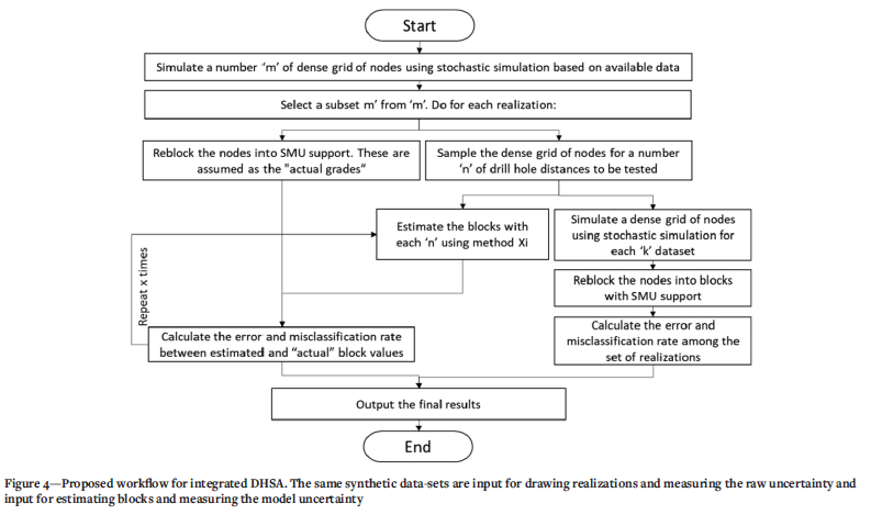
The proposed methodology is an adaptation of the reviewed and widely used methods. Its novelty is the integrated DHSA to support a complete drilling plan from exploration to production models, their limits, and the best geostatistical method for each step. Available DHSA methods and concepts were kept, but algorithms were revised to reduce the computational effort required to run both simultaneously and assure interchangeable results. The integrated DHSA workflow (Figure 4) benefits from the best of both uncertainty workflows that account for local and global uncertainty. The gains arise from the complementarity between raw and model uncertainty, which leads to an increased information level of assessed uncertainties and fewer arbitrary decisions among different methods, scales of decisions, drill-hole spacings, and resource classes.

Computational performance and the results are directly associated with the use of one or all realizations in the DHSA workflow. A guideline is provided by Armstrong et al. (2013) and (Deustch, 2018):

0 The optimal drill-hole spacing and its impact on local parameters, such as the block-by-block error or misclassification rate, may be assessed by a single set or subset of realizations because the variability at specific locations averages out over multiple realizations.

0 In the case of nonlinear relationships or more complex functions, such as a profit expectation or definition of the pit limits, it is recommended to pass all realizations through the transfer function to assess the whole response distribution.

The ideal number of realizations should be defined for each study. Different mineral deposits may require a different number of realizations to model the uncertainty, depending on their grade variability and the scale under analysis. A widely used solution is to measure the convergence of statistics of interest, such as the mean and standard deviations, for increasing values of 'm' and 'n'. This and other approaches may be found in Rossi (1994) and Deutsch and Journel (1998).

 

Applications

Realizing how the practitioner's DHSA premises impact the whole perception of uncertainty is important. Even so, it is not unusual to see drill-hole spacing studies limited to standard strategies for modelling the uncertainty, which may not be suitable for the problems being solved. DHSA should not be exclusively sampling-dependent but should also integrate the geostatistical method used and model purpose into the uncertainty modelling. For example, projects at very early exploration stages support viability studies and technological decisions over the global predictions of grade and metal content. This means that the global gradetonnage proportion is more relevant than the grade uncertainty and selectivity at a mining scale. However, prior exploration drilling may be combined with infill data for estimating production models. During the mining process, local accuracy is fundamental for the final selection. At this stage, minimizing the misclassification of ore and waste blocks is the primary concern. A real optimal sampling plan only may be assessed by an integrated DHSA. Operational conditions usually constrain the sampling programmes in real-world problems. The optimal spacing should consider technical limitations such as the mining scheduling, the grid of blast-hole drilling, or the separation between two consecutive stopes in underground mines. Next, we present some practical considerations on how to apply the proposed solution to fit a unique uncertainty assessment to different DHSA problems.

Example

In this hypothetical case, drill-hole spacing analysis is carried out to define (i) the broadest sample spacing that supports an acceptable misclassification error in production models, and (ii) the sample spacing suitable for classifying the model areas as Measured, Indicated, or Inferred. It is an example applicable to many mining operations, where an integrated study supports the correct geostatistical workflows and drill-hole spacing for each model, as well as defining if the exploration or production team is accountable for the drilling campaign. As discussed, the uncertainties to be modelled in each case come from different sources and it is advisable to treat them with an integrated approach.

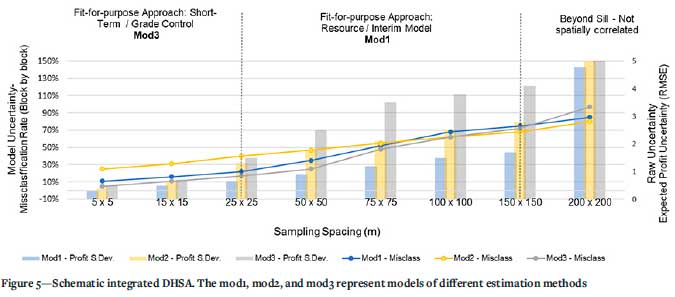
Figure 5 shows a schematic plot for local and global uncertainties as a function of the drill-hole spacing. The plot is an example of how the results of the integrated DHSA should be analysed after following the workflow in Figure 4. The mod1, mod2, and mod³ may represent three different geostatistical methods, e.g., ordinary kriging (OK; Matheron, 1963), sequential Gaussian simulation (SGS; Isaaks, 1990; Deutsch and Journel, 1998), and LUC (Abzalov, 2006), or even a single method adjusted for three different parameters.

When considering a 20% misclassification rate as an acceptable tolerance in Figure 5, mod³ should be selected for grade control. In this case, we see that 25 χ 25 m would be the wider grid that supports the accuracy required for short-term models. For resource categories, i.e., Measured/Indicated/Inferred, as a function of the expected profit uncertainty, the long-term models should be estimated with grids between 25 χ 25 m and 150 χ 150 m. In such cases, mod1 should be selected because it has lower values for the global uncertainty. Models using a grid beyond 150 χ 150 m are of little use from a resource perspective because of their high uncertainty. From this conceptual case, it is quite clear that model uncertainty, if taken from a local or global perspective, changes depending on the evaluation strategy. The essence of the integrated approach is to capture these disparities.

Integrated DHSA applied to a real gold deposit

The studied orebody is part of a world-class gold deposit in the Rio das Velhas greenstone belt located on the north border of the Iron Quadrangle (QF) district, Minas Gerais, Brazil. Geologically, it is classified as a typical association of mafic volcanic rocks, banded iron formation (BIF), carbonaceous phyllite, and micaceous phyllite metamorphosed at greenschist facies conditions (Lobato, 1998). Considering the host rock and the mineral assemblage, Vieira (1987) recognized three main gold mineralization types in the Iron Quadrangle district: (i) rich-pyrrhotite hosted in BIF, (ii) related to pyrite and arsenopyrite replacing the iron layers of banded formations, and (iii) disseminated arsenopyrite in mafic schists.

The case study is developed in an underground mine currently in operation. Long-term models are gradually replaced by detailed grade-control ones as the production and drilling campaign progresses. Depending on how dynamic the operation is, additional interim models may be necessary to support strategic and operational decisions. As the estimates are designed to fit the model purpose, the uncertainty modelling and the DHSA to define the optimal drill-hole spacing are recommended to be likewise.

Simulating the reference scenarios

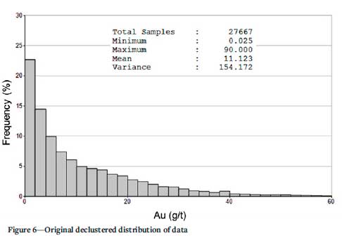
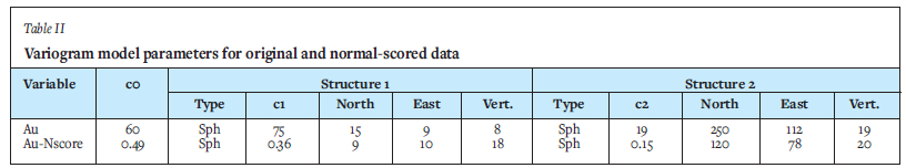
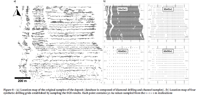
The original data-set came from a depleted area extensively sampled by diamond drill-holes (DDH) and face channels. Figure 6 shows the declustered distribution of the data-set, where the variogram models were fitted to original and normal-score units (Table II).

 

 

The original data was used as SGS input to produce 30 equiprobable realizations in the deposit discretized in a dense 1 χ 1 χ 1 m grid. The sectorized SGS search ellipse was adjusted to fit the ore anisotropy and variogram ranges. The simple kriging was conditioned to 12-64 original samples and up to 36 previously simulated nodes. The 30 resulting realizations satisfactorily reproduced the declustered average grade, distribution, variogram model, and directional anisotropy (Figure 7).

The simulated realizations at the 1 χ 1 χ 1 m grid were used to generate 30 new synthetic data-sets for seven drill-hole spacings to mimic exploration and infill drilling: 5 χ 30 χ 1 m (representing the actual grade control spacing), 10 χ 15 χ 1 m, 20 χ 30 χ 1 m, 30 χ 45 χ 1 m, 40 χ 60 χ 1, 60 χ 90 χ 1 m, and 80 χ 120 χ 1 m along the strike, plunge, and width, respectively (Figure 8). The listed sample spacings are possible considering the technical and operational conditions.

Accounting for the local and global uncertainties

To compute the uncertainty, the integrated workflow (Figure 4) was applied as follows.

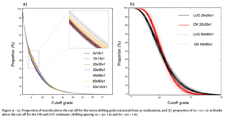
> The 30 'true' realizations were sampled at seven drilling spacings, resulting in 210 synthetic data-sets (Figure 9a).

> Thirty realizations were drawn by the SGS method from the 210 data-sets. The raw uncertainty of each drill-hole spacing was measured as the difference among 1 χ 1 χ 1 m realizations averaged into 10 χ 10 χ 10 m blocks. The synthetic data from SGS was used for the normal score variogram of the original data. The search ellipse orientation and ranges considered the variogram parameters defined in Table II. A sectorized search was conditioned for 12-64 actual samples and up to 36 simulated nodes.

> Ordinary kriging was applied to the 10 χ 10 χ 10 m blocks (Figure 9b). The OK used the original units variogram (Table II), a search ellipse range equal and parallel to this variogram. The sectorized ellipse was conditioned for 16-64 samples, and each block was discretized into 5 χ 5 χ 5 points.

> LUC was applied to the 40 χ 40 χ 40 m panels before 10 χ 10 χ 10 m localization (Figure 9b). The LUC used the original unit variograms (Table II) and search ellipse range equal and parallel to the modeled continuity. The sectorized ellipse was conditioned for 16-64 samples, and each block was discretized into 5 χ 5 χ 5 points.

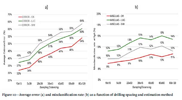
Considering 5 g/t as a theoretical cut-off grade for the reference models, the local accuracy was measured by the misclassification rate of blocks and the average estimation error. The local errors, i.e., the variations between the estimated and the 'actual' values, were quantified by the root mean square error (RMSE). The same was applied to account for global accuracy. We measured the uncertainty of the overall metal-grade relationship for different drill-hole spacings at a range of cut-offs.

Figure 10 presents the DHSA results for local accuracy. The drill-hole spacing (x-axis) was plotted versus the average estimation error and the block's misclassification rate (y-axis). The estimated block was compared to its 'actual' reference value resulting from averaging all simulated nodes inside each block in both cases.

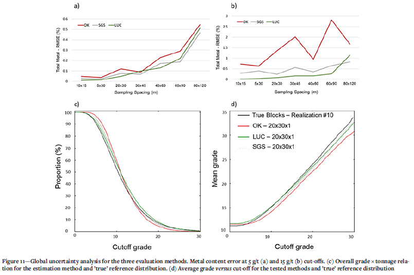
From a global perspective, Figures 11a and 11b show the RMSE for the metal content at 5 and 15 g/t for different drill-hole spacings. Additionally, the overall performance may be tested by comparing the estimated grade-cut-off and grade-tonnage relationships to the 'true' reference model (Figure 11c-d)

This case study highlighted that the errors were not exclusively due to the sample spacing. In contrast, the total model uncertainty arose from different sources, such as the estimation method, parameters, time-frame analysed, support dimension, and data availability.

 

Discussion

The results presented in this case study are consistent with the reviewed literature. While OK provides local estimates with minimum error, the same is not valid from a global perspective. SGS and LUC proved to be better solutions for representing the actual grade-tonnage relationhip and total metal content (Figure 11c-d). LUC incorporates the volume-variance effect into the estimated model. It makes uniform conditioning very effective in reproducing the global grade-tonnage distribution as it reduces smoothing impacts. In this sense, to assess the risks in the metal prediction in cases of sparsely distributed data or over-smoothed kriging, DHSA performed on LUC estimates would provide better uncertainty models.

The metal prediction errors (RSME) from the LUC and SGS methods were smaller than the error associated with the OK estimates (Figure 11a-b). Locally, OK estimates using a 20 χ 30 m drilling grid equal the uncertainty for the SGS simulation with a 10 χ 15 m grid (Figure 10). The metrics for quantifying the local uncertainty are constant, but varying the estimation method leads to different error values. The localization step of the LUC workflow provides SMU estimates from the panel histogram. However, this process may be highly inaccurate from a local perspective (Figure 10a-b). Thus, it is not advisable to perform DHSA studies for measuring the mining selectivity risk without considering the method's characteristics.

The proposed DHSA approach may define limits among the different models and support the selection of geostatistical methods for each application. For grade control models, a higher block-by-block accuracy and lower misclassification rate is required for production and, thus, should be based on OK estimates that support a drilling spacing of 10 χ 15 m or 5 χ 30 m. Considering the maximum uncertainty over the mass analysed at different production scales, a resource model should be defined.

Moreover, one point arising in this study that may be revisited in future studies arises from Figure 10. This figure shows a reasonable linear relationship between the averaged error and the drill-hole spacing. This linearity seems to be a general feature observed in other studies (Koppe, 2017; Usero, Misk, and Saldanha, 2019; Li et al., 2004). If DHSA studies are conducted accordingly, the computational demand could be decreased without overall quality losses. However, that experimental observation must be checked for specific cases or mathematically proved in future studies.

 

Conclusion

The drilling programme, strategy, and their use for supporting grade and geological modelling are some of the most critical activities in any mine. The model uncertainty results from a complex combination of data availability, estimation method, geological features, and the objective function of interest. Therefore, in most cases, DSHA studies require an integrated analysis that considers the problem being addressed under the different applications of the drill-hole data. DHSA workflows available in the literature lead to different results that may not be interchangeable for many problems. Ignoring their differences and choosing any of them without a detailed analysis may result in misleading analysis or suboptimal decisions. We grouped simulation-based DHSA methods as a function of their resulting raw or model uncertainties.

> Raw uncertainty methods provide a means for objective functions, such as the expected profit of a given mine plan, operational dilution, and other engineering

or economic parameters. In these global cases, it is recommended to consider the raw uncertainty, where the entire set of realizations is directly passed through the analysed transfer functions.

> Raw uncertainty, however, is not suitable for assessing the risks of estimating the block grade or its expected misclassification rate. Raw uncertainty workflows ignore method-related outcomes, such as minimum variance optimization, information effects, smoothing effects, and conditional biases. In those cases, the model uncertainty approach better predicts the local uncertainty found in short-term and production models.

The proposed integrated DHSA allows a complete understanding of how the drill-hole spacing responds to the geostatistical method and its limitations, the model purpose, and transfer functions. The proposed method is especially relevant if we consider that resource and grade-control models have different purposes. It offers a wider overview of the uncertainty throughout the life of mine by integrating the short- and long-term perspectives.

The last point to be discussed is the sensitivity of the results to the short-scale behaviour of the modelled variogram, in particular to the nugget effect. This parameter must be carefully defined as it plays a relevant role in DHSA. No optimization study will lead to accurate outputs if the nugget effect is poorly defined. The larger the nugget effect, the larger the point of diminishing returns where the model accuracy is no longer reduced by decreasing the sample spacing. Moreover, a second factor to be considered is the sampling protocol used, how it changes the nugget effect, and the optimal grid. Any optimal sampling strategy needs to consider an optimal and cost-effective ratio between drill-hole spacing and sampling protocol (Abzalov, 2014; Silva and Costa., 2016). Computationally, a higher nugget effect also increases the number of required realizations.

 

References

Abzalov, M.Z. 2006. Localised uniform conditioning (LUC): A new approach for direct modelling of small blocks. Mathematical Geology, vol. 38, no. 4, pp. 393-411.         [ Links ]

Abzalov, M.Z. 2014. Geostatistical criteria for choosing an optimal ratio between quality and quantity of samples - method and case studies. Mineral Resource and Ore Reserve Estimation. The AusIMM Guide to Good Practice. 2nd edn. Australasian Institute of Mining and Metallurgy, Melbourne. pp. 91-96.         [ Links ]

Armstrong, M., Ndiaye, A., Razanatsimba, R., and Galli, A. 2013. Scenario reduction applied to geostatistical simulations. Mathematical Geosciences, vol. 45, no. 2. pp. 165-182.         [ Links ]

Bertoli, O., Casley, Z., Mawdesley, C., and Dunn, D. 2010. Drill hole spacing analysis for Coal Resource classification. Proceedings of the 6th Bowen Basin Symposium 2010, Mackay, Qld, Australia. Geological Society of Australia Coal Geology Group.         [ Links ]

Boucher, A., Dimitrakopoulos, R., and Vargas-Guzman J.A. 2005. Joint simulations, optimal drill hole spacing and the role of stockpile. Geostatistics Banff 2004. Leuangthong O. and Deutsch, C. (eds). Springer, The Netherlands. pp. 35-44.         [ Links ]

Deutsch, CV. 2017. All realizations all the time. Handbook of Mathematical Geosciences: Fifty Years of IAMG. Daya Sagar B.S., Cheng, Q., and Agterberg, F. (eds). Springer. pp.131-142.         [ Links ]

Deutsch, CV. and Journel, A.G. 1998. GSLIB: Geostatistical software library and user's guide. Oxford University Press, New York. 340 pp.         [ Links ]

Drumond, D.A., Amarante, F.A.N., Koppe, VC., and Costa, J. 2019. A chart for judging optimal sample spacing for ore grade estimation: Part II. Natural Resources Research, vol. 29. pp. 551-560.         [ Links ]

Englund, E.J. and Heravi, N. 1993. Conditional simulation: Practical application for sampling design optimization. Proceedings of the Fourth International Geostatistics Congress, vol. 2. Soares, A. (ed.). Kluwer Academic. pp. 613-624.         [ Links ]

Goovaerts, P. 1997. Geostatistics for Natural Resources Evaluation. Oxford University Press, New York. 483 pp.         [ Links ]

Isaaks E.H. 1990. The application of Monte Carlo methods to the analysis of spatially correlated data. PhD thesis. Stanford University. 213 pp.         [ Links ]

Isaaks, E. 2005. The kriging oxymoron: A conditionally unbiased and accurate predictor (2nd edition). Proceedings of Geostatistics Banff 2004, vol. 14. Leuangthong, O. and Deutsch, C.V. (eds.). pp. 363-374. doi: 10.1007/978-1-4020-3610-1.37        [ Links ]

JORC. 2012. Australasian Joint Ore Reserves Committee. Australasian Code for Reporting of Exploration Results, Mineral Resources and Ore Reserves. The Joint Ore Reserves Committee of the Australasian Institute of Mining and Metallurgy, Australian Institute of Geoscientists, and Minerals Council of Australia. http://www.jorc.org/docs/JORC_code_2012.pdf        [ Links ]

Journel A.G. and Huijbregts C.J. 1978. Mining Geostatistics. Academic Press, New York.         [ Links ]

Koppe, VC., Costa, J.F.C.L., Peroni, R.L., and Koppe, J.C. 2011. Choosing between two kinds of sampling patterns using geostatistical simulation: Regularly spaced or at high uncertainty locations? Natural Resources Research, vol. 20, no. 2. pp. 131-142.         [ Links ]

Koppe, VC., Rubio, R.H., and Costa, J.F.C.L. 2017. A chart for judging optimal sample spacing for ore grade estimation. Natural Resources Research, vol. 26, no. 2. pp. 191-199.         [ Links ]

Li, S., Dimitrakopoulos, R., Scott, J., and Dunn, D. 2004. Quantification of geological uncertainty and risk using stochastic simulation and applications in the coal mining industry. Proceedings of Orebody Modelling and Strategic Mining Planning. Australasian Institute of Mining and Metallurgy, Melbourne. pp. 233-240.         [ Links ]

Lobato, L.M. and Vieira, F.W.R. 1998. Styles of hydrothermal alteration and gold mineralization associated with the Nova Lima Group of the Quadrilátero Ferrífero: Part II; The Archean mesothermal gold-bearing hydrothermal system. Revista Brasileira de Geociências, vol. 28, no. 3. pp. 335-336.         [ Links ]

Martínez-Vargas, A. 2017. Optimizing grade-control drill hole spacing with conditional simulation. Minería y Geología, vol. 33, no. 1. pp. 1-12.         [ Links ]

Matheron, G. 1963. Principles of geostatistics. Economic Geology, vol. 58. pp. 1246-1266.         [ Links ]

Okada, R., Costa, J.F.C.L., Rodrigues, A.L., Kuckartz, B.T., and Marques, D.M. 2019. Scenario reduction using machine learning techniques applied to conditional geostatistical simulation. REM - International Engineering Journal, vol, 72, no. 1. pp. 63-68.         [ Links ]

Rossi, M.E. 1994. Of tool makers and tool users. Geostatistics, vol. 7, no. 2. pp. 7-9.         [ Links ]

Rossi, M.E. and Deutsch, C.V. 2014. Mineral Resource Estimation. Springer, Berlin. 332 pp.         [ Links ]

Silva, V.M. and Costa, J.F.C.L. 2016. Selecting the maximum acceptable error in data Minimizing financial losses. Applied Earth Science, vol. 125, no. 4. pp. 214-220.         [ Links ]

Usero, G., Misk, S., and Saldanha, A. 2019. An approach for drilling pattern simulation. Mining Goes Digital: Proceedings of the 39th International Symposium on Application of Computers and Operations Research in the Mineral Industry. CRC Press. pp. 59-66.         [ Links ]

Verly, G., Postolski, T., and Parker, H.M. 2014. Assessing uncertainty with drill hole spacing studies - Applications to Mineral Resources. Proceedings of the Orebody Modelling and Strategic Mine Planning Symposium 2014. Dimitrakopoulos, R. (ed.). AUSIMM Publication Series, vol. 13. Australasian Institute of Mining and Metallurgy, Melbourne. pp. 109-118.         [ Links ]

Vieira, F.W.R. 1987. Gênese das mineralizações auríferas da mina de Raposos. Simpósio de Geologia de Minas Gerais, Belo Horizonte. Sociedade Brasileira de Geologia, anais, vol. 7. pp. 358-368.         [ Links ]

 

 

Correspondence:
B.C. Afonseca
Email: brunocafonseca@yahoo.com.brr

Received: 11 Feb. 2022
Revised: 5 May 2022
Accepted: 6 May 2022
Published: June 2022