WITS SPECIAL EDITION - VOLUME II

 

A version of Gy's equation for gold-bearing ores

 

 

R.C.A. Minnitt

School of Mining Engineering, University of the Witwatersrand, South Africa

 

 

---

SYNOPSIS

The two methods for calibrating the parameters K and α (alpha) for use in Gy's equation for the Fundamental Sampling Error (FSE)-, Duplicate Sampling Analysis (DSA) and Segregation Free Analysis (SFA)-, are described in detail. A case study using identical broken reef material from a Witwatersrand-type orebody was calibrated using the DSA and SFA methods and the results compared. Classically, the form of Gy's equation for the FSE raises the nominal size of fragments given by d_Nto the power of 3. A later modification of Gy's formula raises d_Nto the power α (alpha), the latter term being calibrated with the coefficient K in the DSA and SFA methods. The preferred value of α for low-grade gold ores used by sampling practitioners in the mining industry is 1.5. A review of calibration experiments for low-grade gold ores using the DSA and SFA methods has produced values of K that vary between 70 and 170 and values of a in the range 0.97 to 1.30. The average value for a is shown to be 1, rather than 3 as originally proposed in the classic form of Gy's equation or the industry-preferred 1.5. It is suggested that for low-grade gold-bearing ores the equation for the FSE should raise d_Nto a power of 1. Such an equation for the variance of the FSE greatly simplifies the charac terization of gold ores, now requiring only the calibration of K for a given mass and established fragment size. The implications of the simplified equation for the heterogeneity test are that, provided the fragments have been screened to within a narrow size range, any particular size will return a value for K that is acceptable for use in the sampling nomogram.

Keywords: fundamental sampling error, Gy's equation, gold ore characterization.

---

 

 

Introduction

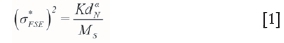
A number of different methods for determining the Fundamental Sampling Error (FSE) have been suggested (Carrasco, 2004; Francois-Bongargon, 1991, 1992a, 1992b, 1993, 1996, 1998a, 1998b; Francois-Bongargon and Gy, 2001; Geelhoed, 2005; Gy, 1973, 1979, 1982; Lyman, 1993; Pitard, 1993; Minnitt and Assibey-Bonsu, 2009; Minnitt, Francois-Bongargon, and Pitard, 2011; Minnitt; 2014). The classic and widely used heterogeneity test for determining the sampling constants was proposed by Gy (Pitard, 1993). It has been described by Carrasco (2005) and Magri (2011), and has been championed by Pitard (2015), but this procedure is not described any further in this paper. Francois-Bongargon (1988a) investigated the changes in the variance of sample assays due to changes in the fragment size, and the way in which this variance can be applied to the determination of the constants K and alpha (a) for use in a modified form of Gy's formula for the FSE shown in Equation [1]. The sampling parameters are substituted into Equation [1] and a graphic, the sampling nomogram, describing the changes in the FSE for different stages of crushing and splitting for a specific ore type at a given grade is compiled.

The method described by Francois-Bongargon (1991), which is generally known as the Duplicate Sampling Analysis (DSA) method, is widely used in the mining industry and has produced consistently useful results in terms of the sampling nomogram that is applied on mining operations. A second method, referred to as the Segregation Free Method (SFA), has also been suggested but is currently not widely applied (Minnitt et al., 2011; Minnitt, 2014).

The primary argument against the DSA method is that the splitting stage before sample analysis requires that 10-20 kg of particulate material be split into 32 samples. Splitting this material, which includes the complete spectrum of fragment sizes from dust to particles up to 19.0 mm in diameter, is thought to introduce grouping and segregation errors that cannot be eliminated or mitigated. The problem of segregation was avoided through a method proposed by Minnitt et al. (2011) and Minnitt (2014), referred to as the Segregation Free Analysis (SFA) method, for calibrating the parameters K and α. The SFA method overcomes the related problems of segregation and ambiguity in regard to the exact size of the fragments, but has been criticized because of its simplicity. Objections raised focus on the single-stage crushing that the material undergoes compared to the multi-stage crushing associated with the DSA method (Minnitt, 2014). The calibration procedures for determining K and α by the DSA and the SFA methods are described and compared. Details of the calculation procedures are almost identical for both methods, but the differences are emphasized.

This paper examines and highlights the differences and similarities in the calibration exercises that have been carried out over the years. As the number of such calibration exercises has increased, there is also growing empirical evidence that the exponent of 1.5 for the nominal fragment size suggested by Francois-Bongargon (1991) and Francois-Bongarcon and Gy (2001) should in fact be unity. This means that the sampling variance is actually a function of the product of the sampling constant Kand the nominal fragment size d_N, divided by the mass. Lyman (1993) proposed a similar equation in which the sampling variance is simply equal to the sampling constant K divided by the sample mass, and has no dependency on the nominal size of the fragments d_N.

 

Preparation of crushed materials for the DSA and SFA methods

Four bins, each containing 400 to 600 kg of run-of-mine gold-bearing ore from the Target, Tshepong, Joel, and Kusasalethu mines, were provided by Harmony Gold Mining Company Limited. The material from each mining operation was handled separately and was spread out to dry, at which stage all fragments larger than 15 cm diameter were examined and identified. These larger fragments, which invariably consisted of sub-rounded dolerite dyke material or fine-grained, non-mineralized hangingwall quartzite, were removed from the lot. A Boyd crusher was used to crush the dried lot to 95% passing 2.50 cm. A total of 333 kg of the broken ore was divided into two lots, one of 75 kg for the DSA experiment and one of 258 kg for the SFA experiment. The 75 kg of broken ore used for the DSA method was split into six series and each of these series was split into 32 individual samples using a rotary splitter. The 258 kg of broken ore for the SFA experiment was split into 15 series and each of these was then split into 32 samples using a riffle splitter. The author sees no difference between the rotary divider and riffle splitter methods.

All samples were submitted for fire assay using a 50 g aliquot. The choice of aliquot was made to improve the precision of the analyses, but was permissible only because of the very good fluxing and fusion characteristics of the Witwatersrand ores. Reduction of the analytical data to provide points on the calibration curves for the DSA and the SFA methods was similar, apart from slight changes in the fragment sizes used on the curves.

 

DSA method

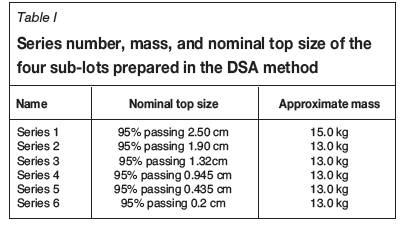
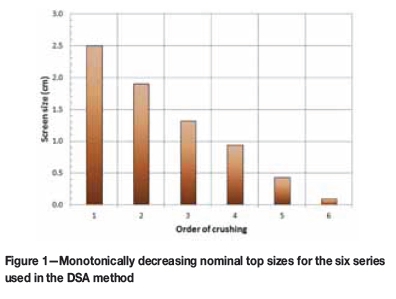
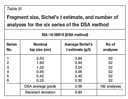
The principal difference between the DSA and SFA methods is in the stages and manner of preparation of the crushed particulate ores for fire assay. The DSA method requires a lot varying from 40 kg to 80 kg, depending on how many series are required. For this particular exercise a series of six sub lots split from the run-of-mine ore from Target mine (Table I), with evenly spread top sizes varying from 2.5 cm to 0.1 mm as shown in Figure 1, was extracted.

 

 

 

 

The first step was to crush the material to a nominal top size of about 95% passing 2.50 cm. This lot was split into six equal, separate sub-lots, each sub-lot being referred to as a series as shown in Figure 2. The first sub-lot of about 12 to 15 kg may be larger than the following sub-lots simply because a greater mass of material is required for larger fragment sizes. This will ensure a better distribution of fragments per sample during the rotary splitting procedure and will reduce the variance of the large fragment sample masses.

 

 

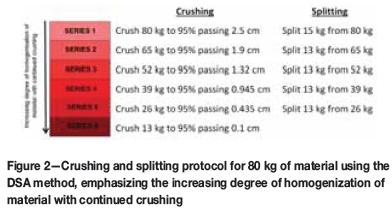
The first of the sub-lots, of 15.0 kg at 2.50 cm, was named Series 1. The remaining five sub-lots (65 kg mass) were recombined and homogenized during crushing to a somewhat smaller sieve size having a nominal top size of 95 % passing 1.90 cm. This lot of about 65 kg was then split into five sub-lots of about 13 kg each, one of which was chosen at random and named Series 2. The remaining four sub-lots were recombined to give a 52 kg lot at 95% passing 1.90 cm. This material was then crushed to a smaller nominal top size, say 95% passing 1.32 cm. The lot was then split into four sub-lots of 13.0 kg each; one was selected and named Series 3. The remaining three sub-lots of about 13.0 kg each were recombined to give a 39 kg lot, which was crushed to 95% passing 0.945 cm and split three ways. One of the sub-lots, 13 kg by mass, was selected and named Series 4. The remaining two sub-lots with a total mass of 26 kg were recombined and crushed to 95% passing 0.435 cm and split to give two equal sub-lots of 13.0 kg each, one of which was named Series 5. The last 13.0 kg sub-lot was crushed to 95% passing 0.20 cm and termed Series 6. The nominal fragment size and mass of each of the different series, 1 to 6, established in this way are shown in Table 1.

Each of the six series was then split into 32 sub-samples of approximately equal mass (39 g) using a rotary splitter or a riffle splitter. Two of the samples were selected at random from each of the Series 1-4 and tested the granulometry for each of the four size fractions, i.e. to check that each size fraction is correctly calibrated. The problems associated with the granulometry test are dealt with by Minnitt et al. (2011). The total mass of material used for the granulometry test is small, about 90-100 g, so the test rarely produces results that unquestionably correlate with the given nominal top size of the lot.

Typically, the DSA method of calibration uses broken ore that is progressively reduced from a top size of about 2.5 cm to fragments around 0.1 cm by crushing. Each fraction that is crushed and split out for use in a series contains a complete distribution of fragment sizes, from the range below the nominal top size to dust. For example, a series with a nominal top size of 1.32 cm will contain a complete distribution of fragments that vary in size from 1.32 cm to fine dust less than 75 μm (Minnitt et al., 2011). Previous experiments using the SFA method have demonstrated that the increase in sample variance times mass with increasing fragment size is positive and linear (Minnitt et al., 2011).

The splitting protocol using a standard riffle splitter is shown in Figure 3.

 

 

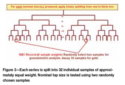
Although it is normal to use three, or at most four, series of split material at different fragment sizes, this particular experiment using the DSA method involved six individual series of material at the fragment sizes listed in Table I.

 

SFA Method

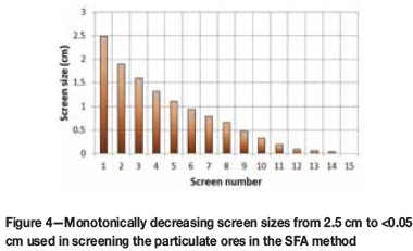
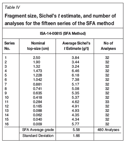
Material preparation for the SFA method is simpler than for the DSA method. In this particular case a mass of about 258 kg of ore from Target mine was crushed to a nominal top size of 2.50 cm and screened through 15 different screens as shown in Figure 4. In a standard SFA experiment four series at different fragment sizes could be used, but in this particular experiment 15 different size fractions were analysed.

 

 

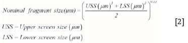
The mass of each screened size fraction is listed in Table II and plotted as a grain size distribution in Figure 5. Each of the series in the SFA experiment at different nominal fragment sizes was then split into 32 samples using a riffle splitter, and each sample was bagged and numbered. The nominal (average) fragment size in micrometres for a fragment passing between two screens can be calculated using Equation [2].

 

 

 

 

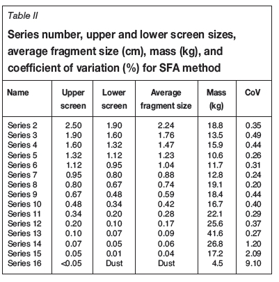
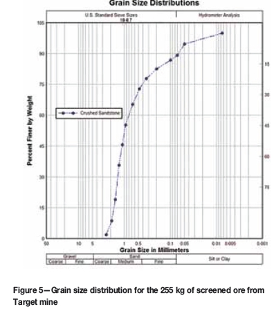
The actual average fragment size for each series retained between two screens as listed in Table II is systematically smaller without any major discontinuities in size. Screening of the broken ore allows the lot to be separated into 15 statistically narrow (clean) size fractions that are then analysed, a method first proposed by Minnitt et al. (2011).

The grain size distribution of the screened ore from Target mine used in this investigation is shown in Figure 5, indicating that about 50% of the material (115.7 kg) is less than 1 mm in diameter.

 

Analysis of the assay data

The lognormal distribution of the assay data required that the means for each series be calculated using a Sichel's t estimate. The summary of the statistics for each series in the DSA and the SFA experiments is shown in Tables III and IV, respectively. The fire assay results for the DSA method are given in Appendix 1, and those for the SFA method in Appendix 2.

 

 

 

 

This data is used in the calibration exercises.

 

Background theory

The following derivation of the equation for the slope, α, and the intercept, K, is presented in Minnitt et al. (2011), but is included here for completeness. The variance in each of the fifteen size fractions analysed must be represented by the same formula if correct estimates of the parameters Kand are to be derived from the calibration curve. The ratio of upper and lower screen sizes r, shown in Equation [3], must be reasonably consistent across all screen sizes.

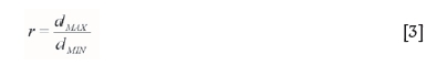
This is indeed the case for most of the larger screen sizes used in this particular SFA experiment, as shown in Figure 6, where r is constrained between 1 and 1.5.

 

 

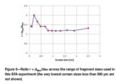
The variance of a sample taken, fragment by fragment, from closely sieved material between d_Minand d_Max is given by Equation [4].

 

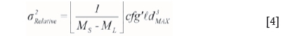
where g' = g'(r) is taken from a curve of the granulometric factor g' versus ratio r = d_Max/d_Minfor closely sieved materials, shown in Figure 7.

 

 

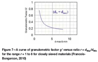
In this experiment the value of r lies between 1 and 1.5, suggesting a g' value of between 0.6 and 0.7 as acceptable for this experiment. The liberation factor I describes the transition between the liberated, calculable variance and the non-liberated one. The term ƒ/g 'd_Max³ represents the average fragment volume in the fraction [d_Min, d_Max]. The smallest size fraction of ratio r in which the mineral is liberated has a d_Max equal to d_ℓ so in the case of the sampling within size fractions of ratio r, the correct liberation factor is:

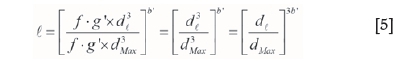
where 0 < b' <1, or, if α = 3-3b', so:

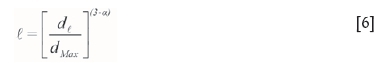
The liberation factor is the ratio of the average fragment volumes at non-liberation and at liberation to a power 3b' in Equation [5], and ƒg'd_Max³ is the average fragment volume in the fraction [d_Min, d_Max]. Generally, the mass of the lot is very much larger than the mass of the sample so that 1/M_L becomes negligible. Substituting Equation [6] into Equation [4] allows us to rewrite Equation [4] as follows:

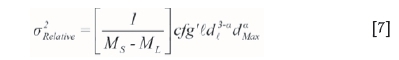
Taking logarithms on both sides of Equation [7], and with the proviso that M_Lis much larger than M_S, allows the equation to be rearranged as follows:

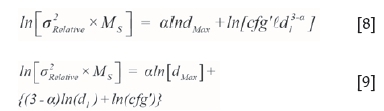
The two variables that are required to compile the calibration curve are then:

So that the slope of the line is given by α, and the intercept is given by:

On this basis it is now possible to extract values for both α and d_t by the fitting of a straight line to the graph (Minnitt et al., 2011).

 

Reduction of the assay data

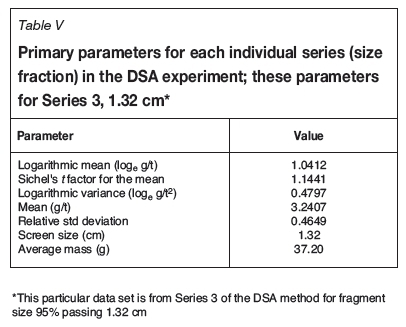
The method of reduction of the 32 fire assay results for each of the series in the DSA and SFA experiments is shown in Table V; this particular data is for the DSA Series 3, samples 1 to 32, at a fragment size of 1.32 cm. The logarithmic mean and variance are presented in this way because the Sichel's t-estimate for the mean of a logarithmic distribution was used to calculate the mean in grams per ton for each of the individual series. Due to calculating the mean in this way, very few data values are eliminated as outliers. The reduction of analytical data for the SFA method is identical to that for the DSA method.

 

 

The data is further reduced to produce the two variables ln(o²*Mass) and ln(d_N) as shown in Table VI.

 

Compilation of the calibration curves for the DSA and the SFA methods

The final reduced data for the six series of the DSA method and the fifteen series of the SFA method is compiled in Figure 8.

 

 

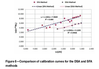
It is noteworthy that the two curves shown in Figure 7 are almost parallel, with slopes of 1.030 for the DSA curve (red) and 1.123 for the SFA curve. The major difference between these curves is the value for the intercepts that they yield: 5.12 for the DSA curve and 7.83 for the SFA curve, which when transformed back from log space gives values of 167.42 g/t² and 2539.1 g/t² respectively.

 

Effect on the nomogram

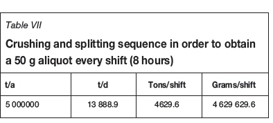
The effect of the differences in K and αfor the DSA and SFA methods and their impact on the sampling nomogram is shown in Figure 8. A typical 5 Mt/a gold mining operation is considered as an example. The mine operates 360 days per annum and three shifts per day, equivalent to about 4.6 million grams per shift (Table VII). Assuming that one assay per shift is required it is necessary to reduce the 4.6 million grams to a single 50 g aliquot for fire assay every shift (8 hours).

 

 

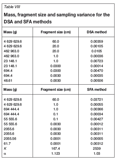
The details of the crushing and splitting stages required to calculate the nomogram of Figure 8 are presented in Table VIII. The sampling variance is calculated using the K and α values substituted into Equation [1].

 

 

The nomograms for the DSA and the SFA methods are compared in Figure 9.

 

 

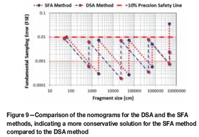
The difference in α is marginal and does not affect the protocol in any significant way, but the difference in K, 167.4 compared to 2539, is significantly large. This difference indicates that the SFA calibration curve produces values of K and α that are more conservative than those with the DSA method. This likewise leads to a more conservative nomogram for the sampling protocol than does the DSA method.

 

Calculation of the liberation size d_ℓ

The liberation size of the gold can be calculated using data derived from the calibration curves for the DSA and the SFA methods. The specific data, together with an explanation of the relevant calculations, is provided in Table IX. It should be noted that the density for gold used in these calculations is that for a gold-silver amalgam with a density of 16 g/cm³.

Having obtained the estimates for αand K we can now calculate values for d_t, the liberation size, using Equation [11].

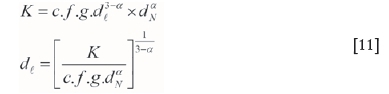
It is important to calculate the liberation size at the nominal fragment size of d_N= 1 cm because at this size K is the correct value and d_N= 1. Substituting values for K and αfor the DSA methods and the SFA method we get:

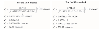
When determining a value for the size of gold grains, i.e. the liberation size, it is essential that all the different size fractions (i.e. the different series) are derived from the same lot, as they are in this particular case. The liberation size d_ℓ of the gold grains was determined at 82 μm for the DSA method and 738 μm for the SFA method. Generally, a liberation size of 738 μm would appear to be too large for typical Witwatersrand gold-bearing ores, with 82 μm being a far more acceptable grain size. However, no work has been completed to establish the exact size distribution of gold in these ores. The liberation size of the SFA lot should probably been verified using another of the mine samples. There is therefore a concern that the SFA method overestimates K; this may be the subject of further work.

 

Accumulated evidence from DSA and SFA calibration experiments

The equation for the estimation of Gy's Fundamental Sampling Error has become firmly entrenched in the minerals industry. It is given by (Francois-Bongargon, 1991):

This equation has been used as a method for defining the calibration curves from which values of αand K can be determined. These values are essential in order to compile sampling nomograms for specific ore types from which a sampling protocol can be designed (Minnitt, Rice, and Spangenberg, 2007; Minnitt and Assibey-Bonsu, 2009; Minnitt et al., 2011).

Since 2009 a number of results from experiments using the DSA and SFA calibration methods have been published, and the equations for the trend lines are listed against the source of the data in Table X. Also shown in Table X is a list of the R² values for the fit of the trend lines to the data. The behaviour of the data-sets that have been accumulated, and which are listed in Appendix 3, is reviewed.

 

 

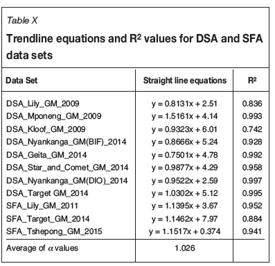
Data listed in Table X is derived from the plots of ln(s²*M_S) versus ln(d_max) for DSA and SFA data-sets that are plotted and shown in Figure 10.

 

 

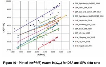
The empirical evidence suggests that the average value for ain gold-related calibration curves shown in Figure 10 is 1.026, which is sufficiently close to unity to suggest that the value should in fact be 1.00. Such a value means that Equation [1] suggested by Francois-Bongargon (1996) should in fact be written as shown in Equation [13].

Such a change in the formula for the FSE results in a considerable simplification in the calculation of the error and in the methods for calibrating a value for Kin Equation [13].

 

Implications for the heterogeneity test

The heterogeneity test (HT) is a standard industry practice that allows the sampling constants, in particular a value for K, to be determined for the purpose of designing and optimizing sample preparation protocols for different types of mineralization. Characterization of mineral size distribution, mineral associations, modes of occurrence, and sampling characteristics of the ores should precede the HT. The standard HT is performed by controlling d_Nto a size as close to 1 cm as possible so that the value of is close to unity; as it turns out the size of fragments between screen sizes of 0.63 and 1.25 cm is 1.05 cm. The mass of each sample is controlled to an exact value so that M_Sis also known exactly. The variance is then calculated from the 100 or so fire assays of samples collected from this particular size range, leaving K as the only unknown which is solved for in Equation [1].

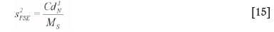
A distinction needs to be drawn between the use of symbols K and C in the equations defining the inherent heterogeneity (of the lot) IHL and the FSE, depending on how the exponent of the nominal fragment size is specified. If the nominal size d has an exponent of 2.5 (d^2.5), or α , where α = 3-x, (d^3-x), the appropriate symbol is K. If the exponent of d is 3(d³), then the appropriate symbol is C. According to Pitard (2009), Gy's earlier literature defined the constant factor of constitution heterogeneity (IH_L) as shown in Equation 14:

Because the liberation factor is a function of d_Nthe constant C, the product of four factors including ℓ, changes as d_Nchanges. For practical purposes it is customary to express IH_L as shown in Equation [14], with little doubt that the exponent of d is α= 3, unless the liberation factor is modelled as a function of d itself. FSE is therefore a function of the sampling constant C, the cube of the nominal size of the fragments (d³_N), and the inverse of the mass of the sample (M_S), giving the familiar formula derived by Gy (1979) and shown in Equation 15:

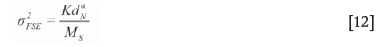
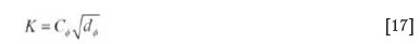
In regard to the HT we define C_Фas the sampling constant for a specific size fraction Ф, i.e. for a single stage of comminution in the sampling process, identified by subscript Ф. The single stage error variance is defined as:

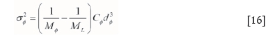
where variables in the equation represent the mass of sample Μφ), mass of lot (M_L), nominal fragment size (d^) and sampling constant (Q) for a specific or single stage variance in a sampling protocol. Equation [16] can be rearranged (Minnitt and Assibey-Bonsu, 2009) to indicate that the sampling constant K does not change from one stage of comminution to another, so that:

However since Equation [13] is now considered applicable for the derivation of FSE, and the exponent of d is now unity, the value for Kshould be the same for any particular size fraction that one may choose to use. No longer is it necessary to use a fragment size close to 1 cm; any fragment size should give the same value for K.

The proposed change in the formula for the FSE also means that the simple HT championed by Gy and Pitard is also simplified and indicates that the only factor needed to establish an acceptable nomogram is a calibrated value for K.

 

Simulated changes in Κand α for the DSA model

A model for low- (1 to 5 g/t) and high- (6 to 22 g/t) grade ores was simulated to examine the behaviour of values for the coefficient K and for the exponent a. For any given fragment size, low-grade ores will generally have lower variance than higher grade ores. The changes in K are large for changes in grade, whereas there are only minor changes in the exponent αfor high- and low-grade ores, as shown in Figure 11.

 

 

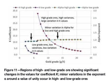
The model shown in Figure 11 indicates that Kdecreases from about 7 to 2 in low-grade ores, and from about 32 to 2 in high-grade ores, as the grade increases from 2 to 22 g/t. Thus the FSE must increase as the grade of the ore increases, meaning that for higher grade ores a sample of larger mass is required. Values for the exponent αchange from 0.96 to 1.03, a marginal change around a value of 1.0, in support of the empirical evidence that a value of unity should be applied in heterogeneity studies and in the construction of nomograms.

Further indications that the value of the exponent in the Francois-Bongargon (1992) version of Gy's formula is unity is provided in Figure 12. Actual data for the exponent from a number of different gold mines where calibration exercises had been carried out are plotted against the corresponding mean grade gold grades in Figure 12.

 

 

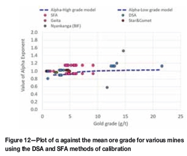
The α values are generally between 0.8 and 1.2 and lie around the α-high grade and α-low grade model lines (dashed) shown in Figure 12. Outliers are present at 0.58 and 1.54, but no clear explanation for these values can be offered. 1.009.

 

Conclusion

This paper compares two different approaches, the DSA and the SFA, to the calibration of the sampling parameters Kand αfor use in the formula proposed by Gy (1979) for the estimation of the Fundamental Sampling Error. The importance of these comparisons is to demonstrate that while they may produce different values for K, the values for the exponent αfor both methods are almost identical and close to unity, as indicated by an analysis of eleven DSA and SFA tests on twelve different gold-bearing ores.

This conclusion has significant implications for future heterogeneity tests in that it indicates that provided the fragment size of the material used for the test is closely screened, any size ratio should produce the same value for the sampling constant K. Furthermore, the nomograms produced for sampling protocols from constants derived from the calibration of K and α will be identical.

 

Acknowledgements

The author acknowledges the permission of the Australasian Institute of Mining and Metallurgy (AusIMM) to publish some of the material presented in a paper at the Sampling 2014 Conference held in Perth. Reviewer's comments resulted in a minor extension to this paper, for which they are thanked.

 

References

Carrasco, P., Carrasco, P., and Jara, E. 2004. The economic impact of correct sampling and analysis practices in the copper mining industry. Chemometrics and Intelligent Laboratory Systems, vol. 74. pp. 209-214.         [ Links ]

Francois-Bongargon, D. 1991. Geostatistical determination of sample variances in the sampling of broken gold ores. CIM Bulletin, vol. 84, no. 950. pp. 46-57.         [ Links ]

Francois-Bongargon, D. 1992a. The theory of sampling of broken ores, revisited: An effective geostatistical approach for the determination of sample variances and minimum sample masses. Proceedings of the XVth World Mining Congress, Madrid, May 1992.         [ Links ]

Francois-Bongargon, D. 1992b. Geostatistical tools for the determination of fundamental sampling variances and minimum sample masses. Geostatistics Troia '92. Kluwer Academic, Dordrecht, The Netherlands. Vol 2, pp. 989-1000.         [ Links ]

Francois-Bongargon, D. 1993. The practice of the sampling theory of broken ores. CIM Bulletin, May 1993.         [ Links ]

Francois-Bongargon, D. 1998a. Extensions to the demonstration of Gy's formula. Proceedings of the CIM Annual Conference, Montreal, May 1998.         [ Links ]

Francois-Bongargon, D. 1998b. Gy's Formula: Conclusion of a New Phase of Research. MRDI, San Mateo, CA.         [ Links ]

Francois-Bongargon, D. 1996. The theory and practice of sampling. A 5-day course presented through the Geostatistical Association of South Africa, Eskom Conference Centre, Midrand, South Africa.         [ Links ]

Francois-Bongargon, D. and Gy, P. 2001. The most common error in applying Gy's Formula in the theory of mineral sampling and the history of the liberation factor. Mineral Resource and Ore Reserve Estimation, the AusIMM Guide to Good Practice. Australasian Institute of Mining and Metallurgy, Melbourne. pp 67-72.         [ Links ]

Geelhoed, B. 2005. A generalisation of Gy's Model for the Fundamental Sampling Error. Proceedings of the 2nd World Conference on Sampling and Blending WCSB2, Sunshine Coast, Old, 10-12 May 2005. Publication Series no. 4/2005. Australian Institute of Mining and Metallurgy, Melbourne. pp 19-25.         [ Links ]

Gy, P.M. 1976. The sampling of broken ores - a general theory. Sampling Practices in the Mineral Industries Symposium, Melbourne, 16 September 1976. Australasian Institute of Mining and Metallurgy, Melbourne. 17 pp.         [ Links ]

Gy, P.M. 1979. Sampling of Particulate Materials. Elsevier, Amsterdam.         [ Links ]

Gy, P.M. 1982. Sampling of Particulate Materials, Theory and Practice. Elsevier. Amsterdam. p. 431.         [ Links ]

Lyman, G.J. 1993. A critical analysis of sampling variance estimators of Ingamells and Gy. Geochimica et Cosmochimica Acta, vol. 57. pp. 3825-3833.         [ Links ]

Minnitt, R.C.A. and Assibey-Bonsu, W. 2009. A comparison between the duplicate series analysis and the heterogeneity test as methods for calculating Gy's sampling constants, K and a. Proceedings of the Fourth World Conference on Sampling & Blending. Southern African Institute of Mining and Metallurgy, Johannesburg.         [ Links ]

Minnitt, R.C.A., Frangois-Bongargon, D., and Pitard, F.F. 2011. The Segregation Free Analysis (SFA) for calibrating the constants K and α for use in Gy's formula. Proceedings of the 5th World Conference on Sampling and Blending WCSB5. Elfaro, M., Magri, E., and Pitard, F. (eds.). Gecamin Ltda, Santiago, Chile. pp.133-150.         [ Links ]

Minnitt, R.C.A. 2014. A comparison of two methods for calculating the constants K and α in a broken ore. Proceedings of Sampling 2014: Where it all Begins, Perth, Western Australia, 29-30 July 2014. Australasian Institute of Mining and Metallurgy, Melbourne. pp. 165-178.         [ Links ]

Pitard, F.F. 1993. Pierre Gy's sampling theory and sampling practice. Heterogeneity, sampling correctness, and statistical process control. CRC Press. 488 pp.         [ Links ]

Pitard, F.F. 2009. Pierre Gy's Theory of Sampling and C.O. Ingamells' Poisson Process Approach, pathways to representative sampling and appropriate industry standards. PhD thesis, Aalborg university, Denmark.         [ Links ]

Pitard, F.F. 2015. The advantages and pitfalls of conventional heterogeneity tests and a suggested alternative. Proceedings of WCSB7, the 7th World Conference on Sampling and Blending, Bordeaux, France, 10-12 June 2005. pp 13-18.         [ Links ]

 

 

Paper received Mar. 2016
Revised paper received Oct. 2016

 

 

Appendix 1- Click to enlarge

 

 

Appendix 2- Click to enlarge

 

 

Appendix 3- Click to enlarge