PAPERS OF GENARAL INTEREST

 

Multivariate geostatistical simulation of the Gole Gohar iron ore deposit, Iran

 

 

S.A. Hosseini; O. Asghari

Simulation and Data Processing Laboratory, School of Mining Engineering, University College of Engineering, University of Tehran, Tehran, Iran

 

 

---

SYNOPSIS

The quantification of mineral resources and evaluation of process performance in mining operations at Gole Gohar iron ore deposit requires a precise model of the spatial variability of three variables (Fe, P, and S) which must be determined. According to statistical analysis there are complex multivariate relationships between these variables such as stoichiometric constraints, nonlinearity, and heteroskedasticity. Due to the impact of these complexities in decision-making, they should be reproduced in geostatistical models. First of all, in order to maintain the compositional and stoichiometric constraints, additive log-ratio (alr) transformation has been applied. In the next step cosimulation, using stepwise conditional transformation (SCT) and sequential Gaussian simulation (SGS) has been used to simulate multivariate data. Through statistical and geostatistical validations it is shown that the algorithms were able to reproduce complex relationships between variables, both locally and globally.

Keywords: additive log-ratios, stepwise conditional transformation, multivariate simulation, iron ore deposit, complex relationship

---

 

 

Introduction

The key steps in mining projects are the quantification of mineral resources, definition of mining reserves, and production scheduling. They rely on the construction of a block model that is used to represent basically the spatial distribution of ore grades (Montoya et al., 2012). The determination of grades and tonnages affects risk assessment and economic evaluation of mining projects. Evaluation of process performance in mining operations requires geostatistical modelling of many related variables (Barnett and Deutsch, 2012). Iron ore quality is characterized by multiple variables: not only the iron grade but also the contaminants that interfere in the subsequent steel manufacturing processes. Consequently, the spatial variability of multiple variables must be determined. Key variables are frequently correlated, and such correlations must be honoured during estimation and simulation. Data from iron ore deposits constitutes compositional data; furthermore, relationships the between assay data are often heteroskedastic.

In order to capture spatial variability and to assess spatial uncertainty, conditional simulation is becoming increasingly popular in the geosciences and the minerals industry for quantifying, classifying, and reporting mineral resources and ore reserves (Journel, 1974; Snowden, 2001). Mineral deposits like iron ore contain several elements of interest with statistical and spatial dependences that require the use of joint geostatistical simulation techniques in order to generate models preserving their spatial relationships. Multivariate modelling can improve the design and planning with respect to traditional models. Additionally, it can help in the assessment of the impact of grade uncertainty on production scheduling (Montoya et al., 2012).

Cosimulation approaches include methods based on the linear model of co-regional-ization, or LMC (Goovaerts, 1997) that can account for the linear (or close to linear) correlations between variables, as the relationship and dimensionality of the data to be modelled may render co-simulation frameworks impractical. Relationships between variables often show complex features such as nonlinearity, heteroskedasticity, and other constraints (Leuangthong and Deutsch, 2003).

One approach is to apply a transformation to the data that removes the relationships, allowing the transformed variables to be simulated independently. Then the variablevariable relationships are restored by back-transformation of the simulated variables. A number of transformation techniques are available that remove these complex features and produce well-behaved distributions that approach Gaussianity. It is highly desirable that the input data to the simulation are standard Gaussian for SGS. There are additional transformations for the de-correlation of variables, allowing independent simulation to proceed without the need for LMC (Barnett and Deutsch, 2012), e.g. principal component analysis (PCA)(Goovaerts, 1993; Hotelling, 1933) and minimum/maximum autocorrelation factors (MAF)(Desbarats and Dimitrakopoulos, 2000; Switzer and Green, 1984), UWEDGE transform (Mueller and Ferreira, 2012), the stepwise conditional transformation (SCT) (Leuangthong and Deutsch, 2003; Rosenblatt 1952) and the projection pursuit multivariate transform (PPMT) (Barnett, Manchuk, and Deutsch, 2014). A shared limitation for linear methods such as PCA and MAF transforms is the poor handling of nonlinear and heteroskedastic features (Barnett et al., 2013). One of the disadvantage of stepwise conditional transformation is that in order to classify data and transform each class, there must be sufficient data to identify a conditional distribution (Leuangthong and Deutsch, 2003). As each technique possesses its own limitations, challenges may arise in choosing the appropriate transforms and the order in which they are applied. Barnett and Deutsch (2012) have proposed a workflow in which transformations are given for the removal of each complexity. No single technique addresses all of the complexities that may exist between the variables of a mineral deposit. Transformations will often be used in chains (Barnett and Deutsch, 2012). In this paper log-ratios (Aitchison, 1982; Pawlowsky-Glahn and Olea, 2004) and STC are used to overcome problems of compositional data and remove the complex features, following the work of Barnett and Deutsch (2012).

The SCT approach has been applied to the modelling of ore deposits such as multivariate simulation of the Red Dog mine (Leuangthong et al., 2006), simulation of total and oxide copper grades in the Sungun copper deposit (Hosseini and Asghari, 2014), and simulation of correlated variables in Yandi Channel iron deposit (De-Vitry, 2010). De-Vitry (2010) recommended that SCT be attempted where significantly nonlinear correlations are present. Log-ratios have also been used to simulate a nickel laterite data-set (Barnett and Deutsch, 2012) and estimate grades in iron ore deposits in Brazil (Boezio et al., 2011). Conditional Gaussian simulations were applied to transformed variables. Back-transformations are executed in the reverse order of which they were applied going forward.

 

Methodology

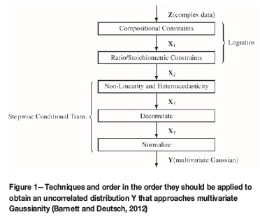
The methodology in the present study is the combination of additive log-ratios (alr) and stepwise conditional transformations proposed by Barnett and Deutsch (2012). Figure 1 shows the proposed order in which multivariate complexities should be addressed to form an uncorrelated multivariate Gaussian distribution. Additive log-ratios (Aitchison, 1982) are used to preserve compositional constraints, and must be applied as the first forward transformation. Then stepwise conditional transformation is used to correct for too-skewed distributions that arise after applying log-ratios and remove the complex features. The major motivation to use SCT in practice is that it is robust when dealing with complex multivariate distributions (Rossi and Deutsch, 2014). Although minimum/maximum autocorrelation factors (MAF) were used to remove correlations between variable elements before simulation, the MAF approach performs poorly with variables that do not demonstrate a linear correlation (Rondon and Tran, 2008; De-Vitry 2010). Butcher and Dimitrakopoulos (2012) have also applied the MAF method for multivariate simulation of the Yandi iron ore deposit, for which the reproduction of the coefficient of correlation between the variables was weak. This contrasts with the STC approach, which is better equipped for handling problematic correlations such nonlinearity and heteroskedasticity. Then sequential Gaussian simulation (SGS), which is efficient and widely used (Lantuejoul, 2002), was performed to simulate transformed variables. Back-transformations are executed in the reverse order to which they were applied going forward.

 

 

Additive log-ratios

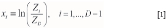
The additive log-ratios transform is used to deal with this constant-sum constraint. The logarithmic transformation must be applied with care when there are zeros for head grade variables. Zeros are obviously problematic, because the logarithm of zero is undefined. The alr transform for D-part composition (Aitchison 1999) is

where x_tis the new variable and Z_irepresents each of the original variables. The back-transformation is

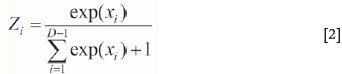
where x_iis logarithmic transformed variable. Directly kriging this log-ratio-transformed data, with a direct back-transform applied results in estimates that are biased. The alternative to direct kriging of log-ratios is to apply a nonlinear approach, in which the conditional distributions of the components are modelled instead of unique values from linear kriging. It has been shown that conditional simulation, where the log-ratio values are transformed into Gaussian values, are valid techniques for dealing with compositional data (Job, 2012).

Stepwise conditional transformation

The STC technique is proposed to transform multiple variables with complex relationships into univariate and multivariate Gaussian with no cross-correlation (Leuangthong and Deutsch, 2003). This method removes all correlations between variables before simulation; thus makes modelling of experimental variograms and simulation faster than conventional cosimulation because cross-variograms and cokriging are not required. The main limitation of the stepwise conditional transformation lies in the need for sufficient data, and this transformation is suitable for low dimensional data-sets (2-4 variables). This transform is identical to the normal score transform for the first variable. For multiple variables, the normal score transformation of the next variable is conditional to the probability class of the preceding variables in the following form:

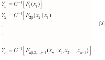
where Y_i, i=1,..., n are multivariate Gaussian variables that are independent at lag distance of zero and are the new variables to be modelled. The transformation ordering for the stepwise conditional transform will affect the reproduction of the variogram from simulation. Thus, the most important variable or the most continuous variable should be chosen as the primary variable. The back-transformation enforces reproduction of the original complex features.

 

Application at Gole Gohar iron ore deposit, Iran

The Gole Gohar iron ore deposit is located at about 55 km southwest of Sirjan in the eastern edge of the Sanandaj-Sirjan structural zone of Iran. The Gole Gohar deposit, comprising six main anomalies and a total reserve of 1300 Mt of high-grade iron ore, is one of the most important economic mineral deposits in Iran. The host rocks include metamorphosed sedimentary and volcanic rocks of the greenschist facies, probably of Upper Proterozoic-Lower Paleozoic age. The mineralization comprises macro-, meso-, and microbanding of magnetite associated with shale, sandstone, and cherty carbonates. The presence of diamictites and phenoclasts in magnetite banding and the host rocks indicates an iron ore association similar to the Rapitan banded iron ore (Babaki and Aftabi, 2006). The Gole Gogar deposit contains 57.2% iron, 0.16% phosphorus, and 1.86% sulphur.

Study area and data

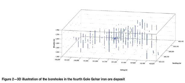
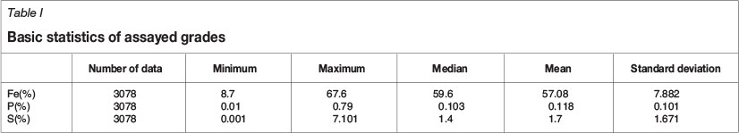
Gol-Gohar iron ore mine anomaly no. 4 is considered in this study. The host rocks are mainly metamorphic rocks, including amphibolite, mica schist, and chlorite schist. Mineralization occurs in both sulphide and oxide forms, and consists of pyrite, pyrhotite, and chalcopyrite as the sulphide minerals, accompanied by other oxide-hydroxide minerals of iron including magnetite, haematite, and limonite. A set of exploration drill-holes is available with an average sampling mesh of 50 m × 50 m. Sample data was composited to 3 m composites and extracted for geostatistical analysis and variography. The assay database comprises 3078 sample intervals from 187 boreholes assayed for iron, phosphorus, and sulphur. A 3D map of drill-hole locations is shown in Figure 2. The basic statistics for these variables are given in Table I. The block model constructed is sufficiently reliable to support mine planning and allow evaluation of the economic viability of a mining project.

Applying transformations to the Gole Gohar data-set

At Gole Gohar Fe%, P%, and S% are variable of interest. The head grades are considered compositional; that is, they are non-negative and sum to 100%. Not all elements in a sample are assayed, therefore the sum of the head grades is less than 100%. In geostatistical modelling, if this constraint is not explicitly imposed it can be violated. A logarithmic transform of four head grade variables is considered, with the fourth variable imposing the 100% constant sum:

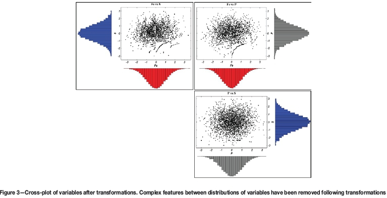
There are few zeros due to the pervasive mineralization to varying extent over the entire deposit. These values have been replaced by the analytical detection limit. The alr transform is used to deal with this constant sum constraint. Z_filter has been used as denominator in Equation [1]. There are now three logarithmic transformed variables, and STC is applied to transform them into Gaussian distributions and remove all correlations between them. For Gole Gohar, Fe is the most important variable, and so the others will be conditioned to it. Due to the spatial continuity, P and S are considered as the second and third variables respectively. Marginal histograms on the bivariate scatter plots of variables after transformations are displayed in Figure 3. The bivariate distributions again exhibit a bivariate Gaussian distribution with essentially zero correlation. Thus, Gaussian simulation techniques can be applied with no requirement for cokriging or to fit a model of co-regionalization.

Simulation of transformed variable

Geostatistical simulations generate a set of images, or 'realizations', as opposed to estimates, which output a single image. The realizations constitute a range of spatial images that are consistent with the known statistical moments (variogram and histogram) of the declustered input data, and in the case of conditional simulations, the data itself. Geostatistical simulations can be used to assess uncertainty over various scales or volumes (e.g. mining production intervals), and can assist in evaluating drill-hole spacing, mining selectivity and blending, and mine financial modelling (Chiles, 2012). In this study, sequential Gaussian simulation or SGS (Isaaks, 1990) has been performed for constructing the realizations. The conditioning samples are migrated to the closest grid node, and a random path is defined through all the grid nodes. Simple kriging is used to construct the conditional Gaussian distribution at each node in the path using the conditioning and previously simulated data. A simulated value is drawn from this conditional distribution and added to the grid node. The next node on the random path is then simulated until all nodes are completed. This process is then repeated to generate n realizations. Each realization contains simulated Fe, P, and S value.

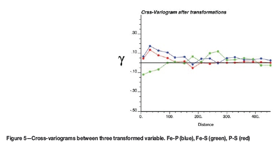
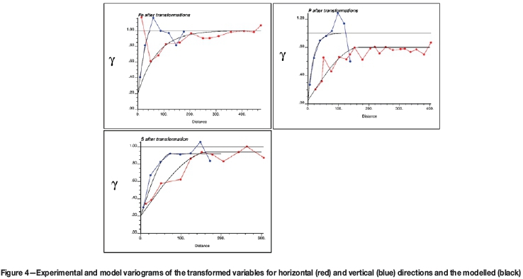
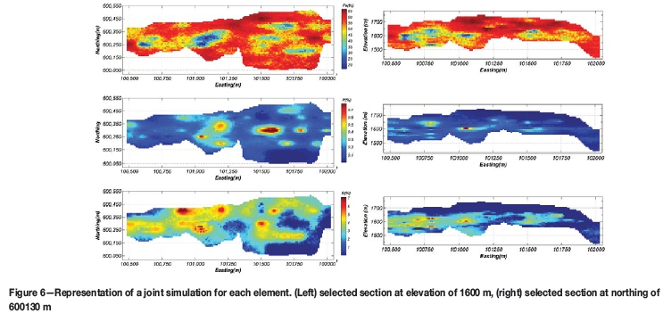
Directional experimental semivariograms were produced for iron, phosphorus, and sulphur after transformations. Experimental and model semivariograms of the transformed variables are shown in Figure 4 and cross-variograms between three transformed variable are shown in Figure 5. The cross-semivariogram takes low values (almost zero). Accordingly, separate modelling of the direct variogram of these variables is undertaken. The total ranges modelled are also utilized to help define the optimum search parameter and search ellipse radii used in the simulation. Applying the two-thirds rule to the total of the variogram range in the search ellipse radius forces the interpolation to use a sample where covariance between samples exists. One joint simulation for the three elements conditional to the drill-hole data (Figure 1) is shown in Figure 6.

 

 

Checking of results

To validate the results, four steps are considered:

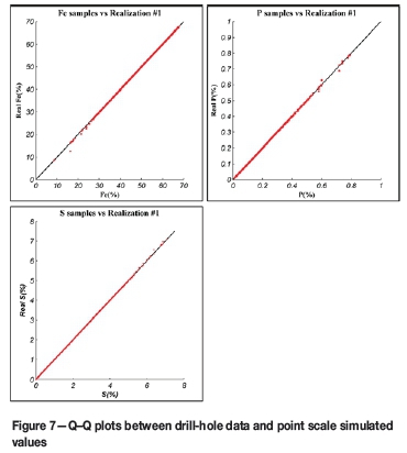
1. Quantile-to-quantile (Q-Q) plots between drill-hole data and simulated values

2. Comparison of drill-hole data and simulation value scatter-plots

3. Comparison of histograms of the sum of three modelled components with the original assays, and simulated values

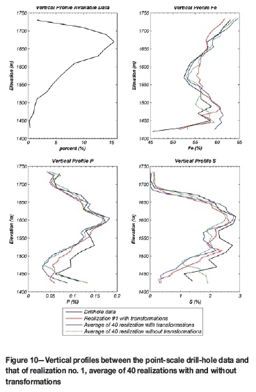
4. Assessment of the vertical profiles of the realizations at block support level.

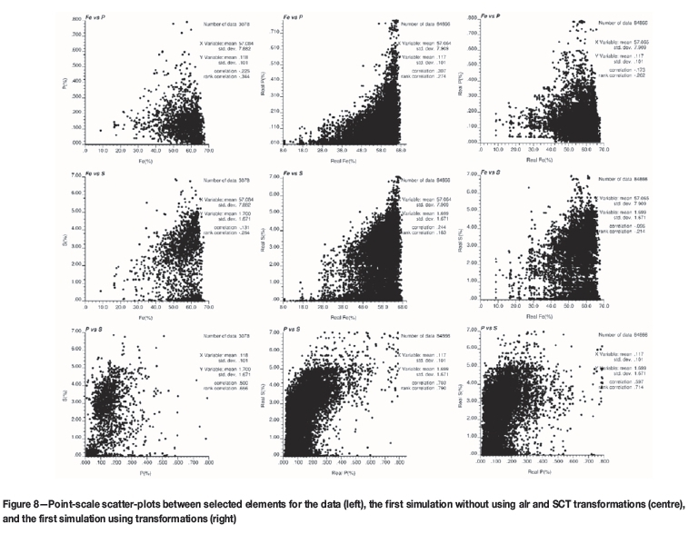
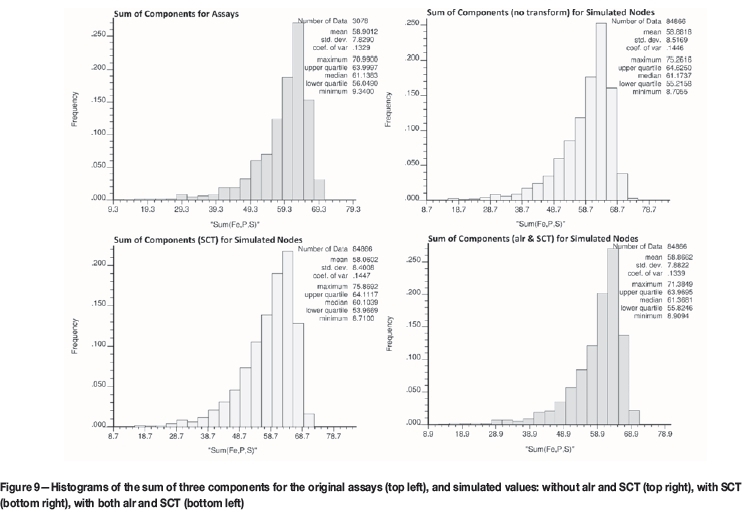
Figure 7 shows that the simulated results reproduce the distributions of the drill-hole data properly. A histogram correction was applied following all back-transformation steps. As a comparison, the point-scale scatter-plots between selected elements for the data, the first simulation without using transformations, and the first simulation using transformations are shown in Figure 8. When the transformations are applied, the shape of the point cloud remains substantially the same, and reproduction of the coefficient of correlation between variables is good. Figure 9 displays histograms of the sum of the three components for the experimental assays and simulated values under three different conditions: (1) without the application of alr or SCT, (2) with the application of SCT, (3) with both alr and SCT. It is observed from the descriptive statistics, especially the maximum value, that the simulated locations with the use of additive log-ratios preserved the compositional constraint explicitly. The simulated locations without the use of alr do not explicitly honour the compositional constraint. Although this issue is demonstrated with only three modelled variables, the results would be much more dramatic when considering the additional components that the mining model would require (Barnett and Deutsch, 2012). In Figure 10, the variation of three elements in the vertical direction is compared. The vertical trends of the elements are an important feature of iron ore deposits (Boucher and Dimitrakopoulos, 2012). The general shape of the profiles is well reproduced in all cases but in elevations 1430 to 1530 m, east of the deposit, there are differences between vertical profile of variables in drill-hole data and the simulation results. These differences are due to the paucity of data.

 

 

 

 

Conclusion

The quantification of mineral resources and evaluation of process performance at the Gole Gohar iron ore deposit requires consideration of three correlated variables (Fe, P, and S). Relationships between these variables show complex features. This paper has shown the practical aspects of an efficient framework for the joint simulation of correlated variables based on a combination of log-ratios and stepwise conditional transformation (proposed by Barnett and Deutsch), and directly generating point-scale realizations. Additive log-ratios were used to honour the compositional constraint, then stepwise conditional transformation was used to correct for the too-skewed distributions that log-ratios create and remove the complex features. The use of this procedure did not require fitting of a LMC for joint simulation of variables. This procedure reproduced the relationships between the variables and histograms of variables well. The realizations are an input for the estimation of mineral resources and ore reserves, and are suitable for mine and plant optimization.

 

References

AiTCHiSON, J. 1999. Logratios and natural laws in compositional data analysis. Mathematical Geology, vol. 31, no. 5. pp. 563-580.         [ Links ]

AiTCHiSON, J. 1982. The statistical analysis of compositional data. Journal of the Royal Statistical Society, Series B (Methodological), vol. 44, no. 2. pp. 139-177.         [ Links ]

Babaki, A. and Aftabi, A.J. 2006. Investigation on the model of iron mineralization at Gol Gohar iron deposit, Sirjan-Kerman. Geosciences Scientific Quarterly Journal, vol. 61. pp. 40-59 (in Persian with English abstract).         [ Links ]

Barnett, R.M. and Deutsch, C.V. 2012. Practical implementation of non-linear transforms for modeling geometallurgical variables. Proceedings of the Ninth International Geostatistics Congress, Oslo, June 2012. Abrahamsen, P., Hauge, R., and Kolbjornsen, O. (eds). Springer, The Netherlands.         [ Links ]

Barnett, R.M., Manchuk, J.M., and Deutsch, C.V. 2014. Projection pursuit multivariate transform. Mathematical Geosciences, vol. 46. pp. 337-359. DOI 10.1007/s11004-013-9497-7        [ Links ]

Boucher, A. and Dimitrakopoulos, R. 2012. Multivariate block-support simulation of the Yandi iron Ore Deposit, Western Australia. Mathematical Geosciences, vol. 44. pp. 449-468.         [ Links ]

Chilès, J.P. and Defliner, P. 2012. Geostatistics: Modeling Spatial Uncertainty. 2nd edn. Wiley, New York. 699 pp.         [ Links ]

Desbarats, A. and Dimitrakopoulos, R. 2000. Geostatistical simulation of regionalized pore-size distributions using min/max autocorrelation factors. Mathematical Geology, vol. 32. pp. 919-942.         [ Links ]

De-Vitry, C. 2010. Simulation of correlated variables. A comparison of approaches with a case study from the Tandi Channel irom Deposit. MSc thesis, University of Adelaide, Australia.         [ Links ]

Goovaerts, P. 1993. Spatial orthogonality of the principal components computed from coregionalized variables. Mathematical Geology, vol. 25. pp. 281-302        [ Links ]

Goovaerts, P. 1997. Geostatistics for Natural Resources Evaluation. Oxford University Press, New York.         [ Links ]

Hosseini, S.A. and Asghari, O. 2014. Simulation of geometallurgical variables through stepwise conditional transformation in Sungun copper deposit, Iran. Arabian Journal of Geosciences. DOI 10.1007/s11004-012-9402-9.         [ Links ]

Hotelling, H. 1933. Analysis of a complex of statistical variables into principal components. Journal of Educational Psychology, vol. 24. pp. 417-441.         [ Links ]

isaaks, E.H. 1990. The application of Monte Carlo methods to the analysis of spatially correlated data. PhD thesis, Stanford University.         [ Links ]

Journel, A.G. 1974. Geostatistics for conditional simulation of orebodies. Economic Geology, vol. 69, no. 5. pp. 673-687.         [ Links ]

Lantuejoul, C. 2002. Geostatistical Simulation: Models and Algorithms. Springer, New York.         [ Links ]

Leuangthong, O. and Deutsch, C.V. 2003. Stepwise conditional transformation for simulation of multiple variables. Mathematical Geology, vol. 35, no. 2. pp. 155-173.         [ Links ]

Leuangthong, O., Hodson, T., Rolley, P., and Deutsch, C.V. 2006. Multivariate simulation of Red Dog Mine, Alaska, USA, CIM Bulletin, May. pp. 1-26.         [ Links ]

Job, M.R. 2012. Application of logratios for geostatistical modelling of compositional data. Master's thesis. University of Alberta.         [ Links ]

Montoya, C., Emery, X., Rubio E., and Wiertz, J. 2012. Multivariate resource modelling for assessing uncertainty in mine design and mine planning. Journal of the Southern African Institute of Mining and Metallurgy, vol. 112. pp. 353-363.         [ Links ]

Mueller, U.A. and Ferreira, J. 2012. The U-WEDGE transformation method for multivariate geostatistical simulation. Mathematical Geosciences, vol. 44. pp. 427-448.         [ Links ]

Pawlowsky-Glahn, V. and Olea, R. 2004. Geostatistical Analysis of Compositional Data. Oxford University Press, New York.         [ Links ]

Rondon, O. and Tran, T. 2008. Multivariate simulation using Min/Max autocorrelation factors: practical aspects and case studies in the mining industry. Geostatistics 2008, Proceedings of the 8th International Geostatistical Congress. Ortiz, J.M. and Emery, X. (eds). Springer-Verlag, Dordrecht. pp. 268-278.         [ Links ]

Rosenblatt, M. 1952. Remarks on a multivariate transformation. Annals of Mathematical Statistics, vol. 23. pp. 470-472.         [ Links ]

Rossi, M.E. and Deutsch, C.V. 2014. Mineral Resource Estimation. Springer, New York. p. 184.         [ Links ]

Snowden, D.V. 2001. Practical interpretation of mineral resources and ore reserve classification guidelines. Mineral Resource and Ore Reserve Estimation-the AusIMM Guide to Good Practice. Edwards, A.C. (ed.). Australasian institute of Mining and Metallurgy, Melbourne. pp. 643-653.         [ Links ]

Switzer, P. and Green, A. 1984. Min/Max autocorrelation factors for multivariate spatial imaging. Technical Report no. 6, Department of Statistics, Stanford University.         [ Links ]

 

 

Paper received Nov. 2014
Revised paper received Apr. 2015.

 

 

© The Southern African Institute of Mining and Metallurgy, 2016. ISSN 2225-6253.