SURFACE MINING CONFERENCE PAPERS

 

Positive risk management: Hidden wealth in surface mining

 

 

J.A. Luckmann

CBS Australia (Pty) Ltd

 

 

---

SYNOPSIS

The purpose of this paper is to introduce an innovative approach to risk management in surface mining operations, namely, positive risk. Traditionally, risk management focused on mitigating losses (negative). Positive risk, on the contrary, reverses the approach and focuses on exploiting a project's inherent benefits (positive).
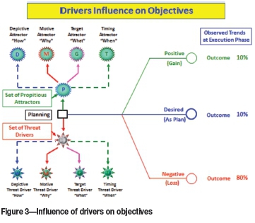
The inability to accurately determine project objectives during the project planning phase and the failure to achieve those objectives during the execution phase is a major problem for any project management in the mining environment.
The advance of computer aided design models for mine planning enables mining engineers to examine various options within a very short time. Employing positive risk management combined with drivers-based risk management when evaluating these options provides an ideal opportunity to investigate areas for improving the mining project's profits. Furthermore, harnessing positive risk returns during the planning phase contributes immensely to the successful achievement of project objectives.
Mining has inherent business risks, which can appear overwhelming when considering the risks associated with a mining project schedule, cost, and safety or resources, etc. The question is - how to manage risks in a surface mining environment, and what process methodologies, work methods, processes, and standards should be used when considering the surface mining risks. Applying the principles of positive risk management to manage surface mining risks is not only relevant, but definitely beneficial to mining projects and to the mining industry as a whole.
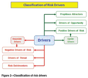
It would certainly be beneficial for risk managers and risk professionals to understand the roles of positive risk 'drivers', also known as 'propitious attractors'. Identifying, analysing, estimating, and understanding the propitious attractors, their behaviour and their influence on project risk events helps considerably during the planning and execution phases. The theoretical and practical knowledge of both sides of the risk - the downside risk (negative risk) and upside risk (positive risk) - can add substantial value to any organization when downside risk is adequately mitigated and upside risk is beneficially exploited.

Keywords: amalgamated risks, conducive risk events, risk drivers, integrated risks, propitious attractors

---

 

 

Introduction

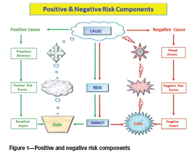
The risk management process is interwoven with shadowy forces which usually influence the outcome of a project, some being negative and some positive. This paper attempts to shed some light on the effects of the negative risk events and the positive risk events and their subsequent outcomes (Yang, Tay, and Sam, 1995).

The ISO 31000 standard, ANZ4360 standard, and some risk professionals have acknowledged the existence of risk drivers (Standards Australia and Standards New Zealand, 2009) and their influence on the outcome of risk events.

If we scrutinize the behaviour of these risk drivers we can observe two types of outcomes, namely, the harmful impacts (Hodder and Rigs, 1994) and the beneficial effects (Furash, 1995). Furthermore, it can be inferred (Luckmann, 2014) that both these forces need consideration during the risk management process because of their opposing characteristics.

The intent of this paper is to define these drives of risk (Alberts and Dorofee, 2009) and to show how to control those forces that beneficially influence the outcome (Simister, 1994).

With that in mind, our immediate attention is to find an adequate and effective means to measure and control the two risk types, namely, the risk detrimentors (negative risk drivers) and the propitious attractors (positive risk drivers).

Therefore, this paper lays emphasis on examining those factors that have harmful and/or beneficial effects on the project objectives.

 

Risk history

Gaius Plinus Secondus (AD 23-79), stated in his 'Natural History', 'Solum certum nihil esse certi (the only certainty is that there is nothing certain). Peter L. Bernstein in his book 'Against the Gods: The Remarkable Story of Risk' describes the history of risk and how risk was through time (Troy, 1995). The history of risk starts with a Hindu-Arabic numbering system that reached the West in the beginning of the 13th century, and could be described as the root of the modern conception of risk as it is known today. The first study of risk began during the Renaissance period. This was the time when people broke free from previous ways of doing things and accepted challenges to open new doors. New discoveries were made, the Earth's resources exploited, and new innovations emerged.

 

 

 

 

In 1654, when the Renaissance was at its peak, Chevalier de Méré, a French nobleman with a taste for both gambling and mathematics, challenged the famed mathematician Blaise Pascal to solve a puzzle about how to divide the stakes in an incomplete game of chance between two players, one of whom is ahead. The puzzle was set forth by Lucas Pacioli, an Italian monk, some 200 years earlier. Pacioli was the inventor of the double entry bookkeeping system, and he also tutored Leonardo da Vinci in the multiplication tables.

The puzzle had confounded mathematicians since the day it was posed by Pacioli, but it was taken seriously up by the Chevalier de Méré. Not even the brilliant Pascal could solve it.

Pascal has to turn to another famous mathematician, Pierre de Férmat, for help and the outcome of a joint project -what could be considered a seventeenth-century version of the game of 'Trivial Pursuit' - was the discovery of the theory of probability. With their solution, Pascal and Férmat created the first practical art of the modern world. Their audacious intellectual leap allowed people for the first time to make forecasts and decisions with the help of numbers. In one fell swoop, the instruments of risk management that had served from beginning of the human history - the stars, the snake dances, the human sacrifices, and genuflections - were rendered obsolete. The modern investor's mantra, the tradeoff between risk and reward, could now become the centerpiece of the decision-making process.

Pascal and Férmat made their breakthrough during a wave of innovation and exploration so powerful that it has been unmatched even in our own era. As the years passed, mathematicians transformed probability theory from a gambler's toy into a powerful instrument for organizing, interpreting, and applying information. As new ideas came along, better quantitative techniques of risk management were developed that could serve as the foundation of modern risk management theory.

By 1725 the English government was financing itself through the sale of life annuities, which were developed by competing mathematicians devising tables of life expectancies. Also in 1725, Swiss mathematician Jacob Bernoulli posited the law of large numbers and the process of statistical inference.

In 1730, the French mathematician Abraham De Moivre discovered the standard deviation and proposed the structure of normal distribution.

A few years later in 1738, Daniel Bernoulli, Jacob's Bernoulli nephew, defined expected utility. Even more importantly, he propounded the idea that 'the utility resulting from any small increase in wealth will be inversely proportionate to the quantity of goods previously possessed'. With that innocent-sounding assertion, Bernoulli combined measurement and intuition into one quantitative concept, hit upon the idea of risk aversion, and laid the groundwork for the basic principle of portfolio management in our own time.

In 1754 an English minister, Thomas Bayes, made a striking advance that demonstrated how to make better informed decisions by mathematically blending new information into old information. Bayes's theorem focused on the intuitive judgment we have about the probability of some event and how we try to understand how to alter those judgments as actual events unfold.

Another discovery, regression to the mean, was made by the English amateur statistician Francis Galton in 1875. Whenever we make any decision based on the expectation that matters will return to 'normal', we are employing the notion of regression to the mean.

In 1952 Harry Markowitz, a young graduate from Chicago University, demonstrated the application of quantified diversification to portfolio management (Luckmann, 2001). This explained why 'putting all one's eggs in one basket' is a very risky strategy and why diversification is a much better risk aversion technique. Markowitz's theory quickly revolutionized corporate finance business decisions, including those made on the Wall Street Stock Exchange.

In 2008, PMI (USA) in 'A Guide to the PMBoK' (Fourth Edition) introduced the concepts of positive and negative risk, and finally on 15 November 2009 the International Standards Organization (ISO) in Geneva, Switzerland introduced the definition of the positive and negative risk events in the ISO 31000 standard.

 

Risk at present

Definition of risk: effect of uncertainty on objectives

► An effect of uncertainty on objective

► Objectives can have different aspects (such as financial, health and safety, and environmental goals) and can apply at different levels (such strategic organization-wide, project, product and process)

► Risk is often characterized by reference to potential events (par. 2.17 of ISO 31000) and consequences (2.18) or a combination of these

► Risk is often expressed in terms of a combination of these consequences of an event (including changes in circumstances) and the associated likelihood (2.19) of occurrence

► Uncertainty is the state, even partial, of deficiency of information related to, understanding or knowledge of an event, its consequence, or likelihood.

Definition of event: occurrence or change of a particular set of circumstances

► An event can be one or more occurrences, and can have several causes

► An event can consist of something not happening

► An event can sometimes be referred to as an incident or accident

► An event without consequences (2.18) can also be referred to as a 'near miss', 'incident', 'near hit', or 'close call'.

Definition ofpropitious attractor. force acting on risk event in a beneficial manner

► Propitious attractor can be one or more attractors acting together, or can be a set of forces acting on a risk (conducive) event beneficially

► A force or set of forces always acting in the upside direction

► Propitious attractor always acting in the opposite direction to risk detrimentors.

Definition of risk detrimentor: force acting on risk event in a harmful manner

► Risk detrimentor can be one or more detrimentors, or can be a set of forces acting together

► A force or set of forces always acting in the downside direction

► Risk detrimentors always acting in the opposite direction to propitious attractors.

Definition of conducive event: uncertainty that, if occurs will affect beneficially one or more outcomes

► Conducive event always results in beneficial outcome

► Conducive event can be driven by one or more propitious attractors.

Definition of negative riskevent: uncertainty that, if occurs will affect negatively one or more outcomes

► Negative risk events always produce a negative outcome

► Negative risk event can be driven by one or more risk detrimentors.

 

History of measurement

Eratosthenes (276 BC -194 BC), Greek astronomer, the 'Father of Measurements', calculated the Earth's circumference around 240 BC.

Eratosthenes used the lengths of shadows to figure out how high in the sky the Sun was in a certain place on a certain day. He knew of another place where there was no shadow at all on the same day, which meant that the Sun was straight overhead. He measured the distance between the two places, and then used geometry to calculate the radius.

Concepts of measurement

'As far as the propositions of mathematics refer to reality, they are not certain; and as far as they are certain, they do not refer to reality.' Albert Einstein, Nobel Prize winner.

'Although this may seem a paradox; all exact science is based on the idea of approximation. If a man tells you he knows a thing exactly, than you can be safe in inferring that you are speaking to an inexact man.' Bertrand Russell, Nobel Prize winner.

The measurements

There are just three reasons why people think that something cannot be measured (Hubbard, 2010). Each of these reasons is actually based on misconceptions about different aspects of measurement:

The definition of measurement itself is widely misunderstood. If one understands what 'measurement' actually means, a lot more things like conducive events and propitious attractors become measurable.

Object of measurement

The thing being measured is not well defined; some sloppy and ambiguous language gets in the way of measurement.

 

 

Methods of measurement

Many procedures of empirical observation are not well known. If people were familiar with some of these basic methods, it would become apparent that many things thought to be immeasurable are not only measurable but may already have been measured.

Definition of measurement

A quantitatively expressed reduction of uncertainty based on one or more observations.

Stochastic approach to measurement

The origin of probability theory lies in physical observations associate with game of chance.

The probability of an event is the number of outcomes favorable to the event, divided by the total number of outcomes, where all outcomes are equally likely.

The calculation of the probability (Ash, 2008) of occurrence must employ the use of data as a critical part of the methodology.

The probability of occurrence is one of the two critical aspects that determines whether a risk is worthy of management (Yang, Tay, and Sum, 1995) or control.

The importance of the Monte Carlo risk measurement is the replacement of single-point deterministic values in a project plan with ranges to reflect uncertainty (Grey, 1995).

Any type of project plan includes fixed values for each element, task or activity, describing the duration, costs, or resources level and allowing the overall project duration, cost, or resources requirement to be simply determined.

The Monte Carlo method is a technique for analysing phenomena by means of computer algorithms that employ, in an essential way, the generation of random numbers.

The Monte Carlo simulation is performed by taking multiple random iterations through the risk model, sampling from input ranges. Each iteration generates one feasible outcome for the project, calculated from a sample of values drawn from the input data.

Multiple iterations produce a set of results reflecting the range of possible outcomes for the project, which reveal the best-case scenario, the worst case, and all circumstances between.

 

 

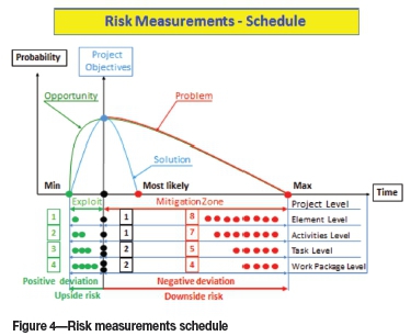
Results are usually presented in a form of an S-curve, a plot of the range of possible outcomes against the cumulative probability of attaining a

Cross-entropy measurement

In 1948 Claude Shannon published a paper titled 'A Mathematical Theory of Communication' which laid foundation for information theory.

Shannon proposed a mathematical definition of information as the amount of uncertainty reduction in a signal, which he discussed in terms of the 'entropy removed by a signal.

To Shannon, the receiver of information could be described as having some prior state of uncertainty. That is, the receiver already knew something and the new information merely removed some, not necessarily all, of the receiver's uncertainty.

The receiver's prior state of knowledge or uncertainty can be used to compute such things as the limits to how much information can be transmitted in a signal, the minimal amount of signal to correct for noise, and the maximum data compression possible.

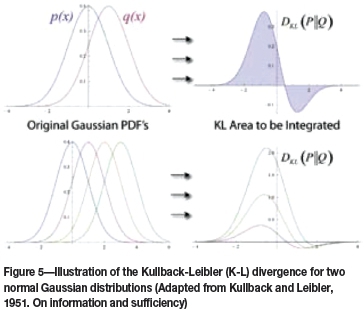
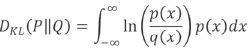
In 1951 Solomon Kullback and Richard Leibrer introduced minimum cross-entropy principle (MinEnt). The Kullback-Leibrer measure is a purely mathematical concept that defines an oriented measure of distance between two probability distributions.

The Kullback-Leibrer (K-L) information divergence (better known as information gain or relative entropy) can be used as a measure of the information gain in moving from a prior distribution to a posterior distribution.

For discrete probability distributions P and Q, the K-L divergence of Q from P is defined as:

 

 

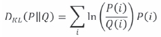
In words, it is the expectation of the logarithmic difference between the probabilities P and Q, where the expectation is taken using the probabilities P. The K-L divergence is defined only if P and Q both sum to 1 and if

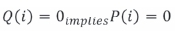
for all i (absolute continuity).

 

 

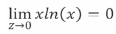
If the quantity 0 ln 0 appears in the formula, it is interpreted as zero because,

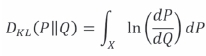
For distributions P and Q of a continuous random variable, K-L divergence is defined to be the integral.

where p and q denote the densities of P and Q.

More generally, if P and Q are probability measures over a set X, and P is absolutely continuous with respect to Q, then the K-L divergence from P to Q is defined as

In 1957 Edwin Jaynes introduced maximum entropy principle (MaxEnt), which is the method of statistical inference when information about a problem is presented in terms of averages, such as mean or variance.

Central to the MaxEnt thesis is the principle of maximum entropy, which states that given certain 'testable information' about a probability distribution, for example particular expectation values, but which is not in itself sufficient to uniquely determine the distribution, one should prefer the distribution that maximizes the Shannon information entropy.

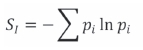
This is known as the Gibbs algorithm, having been introduced by J. Willard Gibbs in 1878 to set up statistical ensembles to predict the properties of thermodynamic systems at equilibrium. It is the cornerstone of the statistical mechanical analysis of the thermodynamic properties of equilibrium systems.

A direct connection is thus made between the equilibrium thermodynamic entropy S_Th, a state function of pressure, volume, temperature, etc., and the information entropy for the predicted distribution with maximum uncertainty conditioned only on the expectation values of those variables:

k_B, Boltzmann's constant, has no fundamental physical significance here, but is necessary to retain consistency with the previous historical definition of entropy by Clausius (1865).

However, the MaxEnt school argues that the MaxEnt approach is a general technique of statistical inference, with applications far beyond this. It can therefore also be used to predict a distribution for 'trajectories' Γ over a period of time by maximizing.

This 'information entropy' does not necessarily have a simple correspondence with thermodynamic entropy, but it can be used to predict features of non-equilibrium thermo-dynamic systems as they evolve over time.

This uncertainty reduction point of view is what is critical to business. Major decisions made under a state of uncertainty, such as whether to approve large information technology (IT) projects or new product development, can be made better, even if just slightly, by reducing uncertainty. Such an uncertainty reduction can be worth millions.

So a measurement does not have to eliminate uncertainty after all. A mere reduction in uncertainty counts as a measurement and possibly can be worth much more than the cost of a measurement.

 

Case study: shaft sinking

Context

Two round concrete lined shafts of 5 m and 6 m diameter restarted the sinking operation process; the principal shaft PA from the 182 m level and the auxiliary shaft PX from the 141 m level.

Due to a fatal accident the shaft sinking operation was terminated by Court order, except for dewatering of the principal and auxiliary shafts to avoid flooding.

As a result of the recommendations made by the accident investigating commission, the Court allowed the resumption of shaft sinking operations in both shafts.

However, over a year of delays and new safety measures imposed by the Court order made a severe impact on the shaft sinking operational performance.

Problem

Three months after the shaft sinking operation was resumed, the performance was significantly below that prior to the accident. Therefore, it was necessary to commission a team of risk specialist to assess and review the project risk management on site.

Risk model

The risk model of the underlying dynamics of the risk detrimentors and propitious attractors was constructed to depict their influence on the risk events.

This risk model was developed by CBS Australia. The purpose of this model was to accommodate the lowest WBS levels to create suitable base, thus enabling more accurate identification of the risk drivers and propitious attractors.

On the work package level, threat drivers and propitious attractors were identified more accurately and measured exactly.

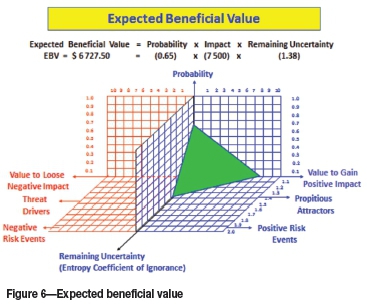
The centrepiece of this model was an introduction of three-dimensional approaches to measurement of the risk events, where the value to lose (VTL) was balanced with the value to gain (VTG).

In order to enhance the risk assessment process the coefficient of ignorance calculation and the factor of remaining uncertainty were also used to enhance the risk measurement and control.

Risk events on component, task, and work package levels were simulated using Palisade Software @RISK 6.2, based on the Monte Carlo method (Schuyler, 1994).

The integrated risk assessment model is depicted in Figure 6.

 

 

Risk identification

Identification of risks encompassed (Frigenti and Kitching, 1994) the process of finding, recognizing (Hulett, 2013) and describing both risk events on the four risk breakdown structure (RBS) levels. Threat drivers (risk detrimentors) and opportunity drivers (propitious attractors) were accurately identified (Luckmann, 2014) on the lowest RBS level. The risks events on the first RBS level (element level) are depicted in Table I.

 

 

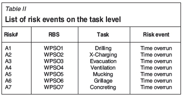
The risk events from the second RBS level (task level) are presented in Table II.

 

 

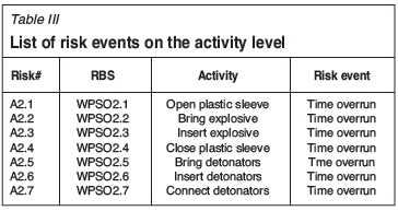
The risk events description on the third RBS level ( activity level) are given in Table III.

 

 

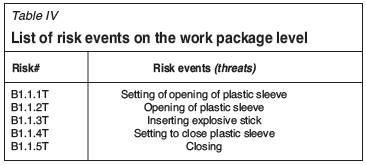
The risk events (threats) description on the fourth RBS level (work package level) is given in Table IV.

 

 

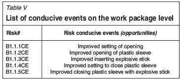
The risk conducive events (opportunities) description on the fourth RBS level (work package level) are given in Table V.

 

 

Risk analysis

Risk events (negative and positive) were subjected to analysis on the fourth level of the risk breakdown structure (RBS).

The risk analysis on the first RBS level, the element level, provided number of negative risk events and positive risk events in the project.

Risk analysis on the second RBS level, the task level, clearly indicated the magnitude of the value to lose (VTL) and extent of the value to gain (VTG).

Risk analysis on the third RBS level, the activity level, ascertained the size of VTL and VTG and depicted the set of risk drivers and the set of propitious attractors.

Analysis of risk drivers (Alberts and Dorofee, 2009) and risk events on the fourth RBS level, the work package level, depicted the risk drivers and risk events and described (Luckmann, 2014) how those drivers and events were measured by the use of Monte Carlo simulation method.

Propitious attractors and favourable events analysis on the fourth RBS level, the work package level, portrayed the propitious attractors and favourable events and how those attractors and favourable events were measured. Application of the Monte Carlo simulation method indicated where the random numbers were generated by the Fibonacci generator (pseudo random generator).

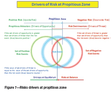
The risk drivers at the pessimistic zone and propitious attractors at the optimistic (propitious) zone are depicted in Figure 7.

 

 

Risk evaluation

The risk-negative events and risk-positive events (Aven, 2011) were evaluated on the fourth RBS level by the use of Monte Carlo simulation techniques.

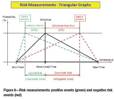
In both cases VTL and VTG were computed. The risk model for the Monte Carlo simulation is given in Figure 8.

 

 

The threat drivers were simulated by Monte Carlo random generators (Luckmann, 2001) and the propitious attractors were subjected to application of the Fibonacci random generator (Froot, Scharftein, and Stein, 1994).

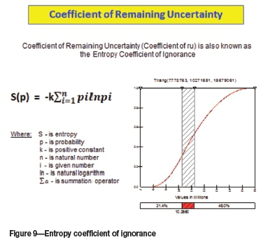
The coefficient of remaining uncertainty (Kapur and Kesavan, 1992) was simulated and results are presented in Figure 9.

 

 

Discussion of results

Twelve favourable risk events (positive) and twelve propitious attractors were identified as economically viable and to be beneficially exploited. It was recommended that the client create the beneficial response plan (BRP) and implement it.

Seventeen negative risk events and seventeen risk detrimentors were posing serious impact on the shaft sinking operation, and generation of a risk response plan (RRP) was recommended. These negative risk events were mitigated and the magnitude of the risk detrimentors was substantially decreased.

 

Conclusions

Rising costs and fierce competition in the global market require incessant search for new opportunities and novel approaches to risk management.

From this case study, it becomes evident that risk detrimentors acting on the negative risk events can be measured, controlled, and mitigated.

The results also indicated that a new unexploited source of project time and cost savings lies inherently in the positive risk (favourable events).

The propitious attractors and favourable events can also be measured and beneficially exploited.

The examples presented in this paper demonstrate the potential opportunities that can be exploited by putting in place positive risk methods to tap an entirely unexploited domain in the project risk management.

 

Acknowledgements

The author would like to thank the client and the project team for allowing CBS Australia consultants access to conduct this complex information-gathering exercise on all the aspects of the shaft sinking operation.

The author takes this opportunity to thank CBS Australia staff for the intellectual and conceptual contributions to conducting measurements in difficult shaft-sinking conditions.

Special thanks to CBS Australia's International Consultants for their diligence, outstanding professional performance, and intellectual contribution.

 

References

Alberts, A.J. 2008. Assessing Risk and Opportunity in Complex Environments, Mission Assurance Analysis Protocol, MAAP. pp.17-19.         [ Links ]

Alberts, C.J. and Dorofee, A.J. 2009. A Framework for Categorizing Key Drivers of Risk. Technical Report CMU/SEI-2009 -TR - 007 ESC -TR - 2009 - 007 http://www.sei.cmu.edu. pp. 11-23.         [ Links ]

Ash, R.B. 2008. Basic Probability Theory. Dover Edition, Department of Mathematics, University of Illinois. pp. 21-32.         [ Links ]

Aven, T. 2011. Quantitative risk assessment: the scientific platform. Cambridge University Press. pp. 34-35.         [ Links ]

Atkinson, R. 1999. Project management: cost time and quality, two best guesses and a phenomenon, it's time to accept other success criteria. International Journal of Project Management, vol. 17, no. 6. pp. 237-242.         [ Links ]

Standards Australia and Standards New Zealand. 2009. Australian/New Zealand Standard AS/NZS 4360: Risk Management. Homebush, NSW and Wellington. New Zealand.         [ Links ]

Frigenti, E. and Kitching, J. 1994. Risk identification a key to project success. Project Pro, July pp. 31-35.         [ Links ]

Froot, K.A.S., Scharftein, D.S., and Stein, J.C. 1994. A framework for risk management. Harvard Business Review, November/December. pp. 91-100.         [ Links ]

Furash, E.E. 1995. Risk challenges and opportunities. Bank Management, May/June. pp. 34-41.         [ Links ]

Grey, S. 1995. Practical Risk Assessment for Project Management. Wiley. pp. 34-43.         [ Links ]

Hillson, D. 2004. Effective Opportunity Management for Projects, Exploiting Positive Risk. Taylor & Francis, New York. pp.14 -18.         [ Links ]

Hodder, J.E. and Riggs, H.E. 1994. Pitfalls in evaluating risky projects. Project Management. pp. 9-16.         [ Links ]

Hubbard, D.W. 2010. How to Measure Anything, Finding the Value of 'Intangible' in Business. Wiley, Hoboken, New Jersey. p. 44-47.         [ Links ]

Hulett, D.T. 2013. The Risk Driver Approach to Project Schedule Risk Analysis. A webinar presented to the College of Performance Management, 18 April 2013. pp. 14 -16.         [ Links ]

International Standards Organization. 2009. ISO 31000, Risk Management - Principals and Guidelines, First Edition. Geneva.         [ Links ]

Kapur, J.N. and Kesavan, H.K. 1992. Entropy Optimization Principles with Application. Academic Press. pp 10-12.         [ Links ]

Luckmann, J.A. 2001. Project cost risk analysis using Monte Carlo simulation: a case study. Proceedings of the Final Year Symposium, University of Pretoria, 17-18 October 2001. pp. 135-146.         [ Links ]

Luckmann, J.A. 2001. Risk Analysis in Project Cost, Schedule, and Performance by Modelling, Simulation, and Assessment: A Case Study. Masters dissertation, University of Pretoria. pp. 51-57.         [ Links ]

Luckmann, J.A. 2014. Positive risk management: hidden wealth in surface mining. Surface Mining 2014 Conference, Nasrec Expo Centre, Johannesburg, 16-17 September 2014. p. 113-124.         [ Links ]

Simister, S.J. 1994. Usage and benefits of project risk analysis and management. International Journal of Project Management, vol. 12, no. 1. pp. 5-8.         [ Links ]

Schuyler, J.R. 1994. Decision analysis in projects: Monte-Carlo Simulation. PMNET Work, January. pp. 30-36.         [ Links ]

Troy, E. 1995. A rebirth of risk management. Risk management, July. pp. 71-73.         [ Links ]

Vose, D. 1996. Quantitative Risk Analysis: A Guide to Monte Carlo Simulation Modelling. Wiley, Hoboken, NJ. pp. 32-37.         [ Links ]

Yang, K.K. 1995. Theory and methodology: a comparison of stochastic scheduling rules for maximizing project net present value. European Journal of Operations Research, vol. 85, no. 2. pp. 327-339.         [ Links ]

 

 

This paper was first presented at the, Surface Mining 2014 Conference, 16-17 September 2014, The Black Eagle Room, Nasrec Expo Centre, Johannesburg, South Africa.