DANIE KRIGE COMMEMORATIVE EDITION - VOLUME III

 

Cokriging of compositional balances including a dimension reduction and retrieval of original units

 

 

V. Pawlowsky-Glahn^I; J.J. Egozcue^II; R.A. Olea^III; E. Pardo-Igúzquiza^IV

^IDept. Informàtica, Matemàtica Aplicada i Estadistica, U. de Girona, Girona, Spain
^IIDept. Matemàtica Aplicada III, U. Politècnica de Catalunya, Barcelona, Spain
^IIIUnited States Geological Survey, Reston, VA, USA
^IVInstituto Geológicoy Minero de España, Madrid, Spain

 

 

---

SYNOPSIS

Compositional data constitutes a special class of quantitative measurements involving parts of a whole. The sample space has an algebraic-geometric structure different from that of real-valued data. A subcomposition is a subset of all possible parts. When compositional data values include geographical locations, they are also regionalized variables. In the Earth sciences, geochemical analyses are a common form of regionalized compositional data. Ordinarily, there are measurements only at data locations. Geostatistics has proven to be the standard for spatial estimation of regionalized variables but, in general, the compositional character of the geochemical data has been ignored. This paper presents in detail an application of cokriging for the modelling of compositional data using a method that is consistent with the compositional character of the data. The uncertainty is evaluated by a Monte Carlo procedure. The method is illustrated for the contents of arsenic and iron in groundwaters in Bangladesh, which have the peculiarity of being measured in milligrams per litre, units for which the sum of all parts does not add to a constant. Practical results include maps of estimates of the geochemical elements in the original concentration units, as well as measures of uncertainty, such as the probability that the concentration may exceed a given threshold. Results indicate that probabilities of exceedance in previous studies of the same data are too low.

Keywords: geostatistics, linear coregionalization model, compositional data, equivalent class, geochemistry, detection limit, groundwater, Bangladesh.

---

 

 

Introduction

Compositional data consists of observations recording relative proportions in a system. The sample space is a simplex, which has an algebraic-geometric structure different from that of real space, known as Aitchison geometry of the simplex (Pawlowsky-Glahn and Egozcue, 2001; Pawlowsky-Glahn et al., 2015). A subcomposition is a subset of all possible proportions. An example of compositional data is the percentages of different minerals in a rock specimen. For such a type of data, a first obvious property is that, when measured without error, the sum of the proportions of all components, known as parts in the compositional literature (in this case minerals), adds up to 100 per cent. In some other less frequent cases, such as the one of our interest, the sum of all proportions is not constant, requiring a slightly different approach. When several specimens have been collected and analysed over some geographical area, usually there is the interest of analyzing the fluctuations in composition both in variable and geographical space.

The exact nature and properties of compositional data have been a source of prolonged misunderstanding and neglect. Pearson (1897) published the first scientific study pointing to peculiar statistical properties when analysing ratio variables, not displayed by multiple variables varying in real space. However, his insights were mostly ignored for more than half a century until Chayes (1960, 1962, 1971, 1975, and 1983) devoted serious effort to advance the analysis of petrographic data. Compositional data analysis, however, would not take off until Aitchison (1982) introduced the logratio approach and published his monographs (1986).

Owing to the different properties from conventional multivariate data, the approach to compositional data analysis has been to convert the compositional variables to conventional real variables. The development of special statistics honoring the compositional peculiarities has proven to be a demanding endeavour showing no significant results. The strategy of representing compositions using logratio coordinates of the simplex (Mateu-Figueras et al., 2011) makes possible the rigorous application of the standard methods of statistics, thus avoiding development of a parallel branch of statistics. The approach sometimes requires back-transforming the results of the analysis in coordinates to the original compositional proportions or concentrations. The literature sadly contains numerous examples in which compositional data is modelled implicitly under false assumptions, such that the parts vary between -∞ to +∞, and that they obey Euclidean geometry. The consequences of violating these assumptions are rarely evaluated and go unchecked. In our case, we are interested in applying the methods of geostatistics, which has become the prevalent approach to mapping when taking into account uncertainty. An early publication on the subject of spatial estimation of compositional data is that of Pawlowsky (1984), later expanded into a monograph (Pawlowsky-Glahn and Olea, 2004). Developments in recent years, such as the formulation of balances (Egozcue et al., 2003: Egozcue and Pawlowsky-Glahn, 2005) (see Equation [3]), make it advisable to revisit the subject.

Geochemical surveys are one of the most common sources of compositional data in the Earth sciences. Survey results are reported as the chemical concentrations of several minerals, oxides, chemical elements, or combinations thereof, as measured in the laboratory. Analytical data that are collected and reported is selective, never including all the elements in the periodic table; therefore, the data available for study covers only a subcomposition of the entire system. For multiple reasons, the interest of the analysis concentrates even further on a detailed account of only a few of the compositional parts. This is the subject of our contribution. The modelling of subcompositions requires additional cautions not necessary for the modelling of whole systems (Pawlowsky, 1984). The first caution is that reduction of dimension implies some form of projection of the data-set preserving the original proportions, a topic not addressed in previous contributions, such as Tolosana-Delgado et al. (2011). Consistent with the compositional approach, the projection is preferred to be an orthogonal projection in the Aitchison geometry of the simplex (Egozcue and Pawlowsky-Glahn, 2005; Egozcue et al., 2011; Pawlowsky-Glahn et al., 2015). The second point concerns the presentation of results of cokriging. Interpolated maps of a single part, using the units in which the original composition was expressed, are a common interpretative tool that is not directly provided by a compositional analysis. The way to obtain these single-part maps from a compositional cokriging is also analysed for the first time in a spatial context, following an analysis in the nonspatial context (Pawlowsky-Glahn et al., 2013).

We borrowed a public domain data-set to practically illustrate our methodology. We selected a survey of environmental importance conducted in the 1990s as a joint effort by the British Geological Survey and the Department of Public Health Engineering of Bangladesh (British Geological Survey, 2001a, b). Many authors have modelled this Bangladesh survey, none of whom took into account the compositional nature of the data, e.g. Anwar and Kawonine (2012), Chowdhury et al. (2010), Gaus et al. (2003), Hassan and Atkins (2011), Hossain and Piantanakulchai (2013), Hossain and Sivakumar (2006), Hossain et al. (2007), Pardo-Igúzquiza and Chica-Olmo (2005), Serre et al. (2003), Shamsudduha (2007), Shamsudduha et al. (2009), Yu et al. (2003). Moreover, the data-set has the peculiarity that instead of part per million, the concentrations are reported as milligrams per litre, a practice shown below to require a special final calibration to have the final results in the original units of measurement.

Following the original environmental interest of the survey, we selected arsenic and iron as the two chemical elements of interest. The main objectives of our paper are to (a) provide a summary review of cokriging for the stochastic mapping of compositional regionalized variables; (b) present and justify the multiple stages of preparation for compositional data required for a proper spatial estimation, in particular projection strategies for dimension reduction; (c) provide a novel back-transformations approach required for the display of results in the original units of concentration; and (d) model the uncertainty in the mapping.

 

Methodology

Aitchison geometry for compositional data

Compositional data comprises parts of some whole. Consequently, multiplication by a positive real constant does not change the knowledge that can be extracted from the data. Thus, the data can be modelled by equivalence classes of vectors whose components are proportional (Barceló-Vidal et al., 2001). These equivalence classes contain a representative for which their components add to a given constant κ>> 0, allowing a general approach independently if the sum of all parts is constant or not. All these representatives form the sample space of compositional data, the D-part simplex, S^D,defined as

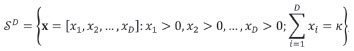
where κ>is the closure constant, e.g. κ>=10⁶ in the case of units of parts per million. All measurements done for the same specimen define a vector of values. In a tabulation, the standard practice is to have data registered row-wise and parts or variables column-wise.

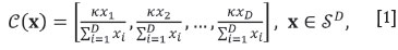
The simplex, with the operations perturbation and powering, and the inner product, called the Aitchison inner product, is a D -1-dimensional Euclidean vector space (Billheimer et al, 2001; Pawlowsky-Glahn and Egozcue, 2001). For C the closure operation,

and the perturbation is defined as

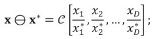
with inverse operation or subtraction

powering is defined as

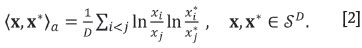
and the Aitchison inner product as

The corresponding squared distance

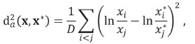
satisfies standard properties of a Euclidean distance (Martin-Fernandez et al., 1998), such as

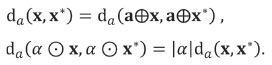
The corresponding geometry is known as Aitchison geometry, and the subscript a is used accordingly (Pawlowsky-Glahn and Egozcue, 2001). The inner product (Equation [2]) and its norm, ||x||_α>= √〈x, x〉_α>, ensure the existence of orthonormal bases. Orthonormal bases and their respective coordinates are important, as standard methods can be applied to the coordinates without restrictions or constraints. This implies that all compositional results and conclusions attained using coordinates do not depend on the specific basis of the simplex used to model compositions in coordinates. This is the core of the principle of working on coordinates (Mateu-Figueras et al., 2011).

In practice, user-defined, simple, specific bases of the simplex can be used. The user defines a sequential binary partition (SBP) (Egozcue and Pawlowsky-Glahn, 2005, 2006) that assigns a set of D-1 coordinates, called balances, to each data location. Balances are normalized logratios of geometric means of groups of parts, and they belong to the family of isometric logratio ( ilr) transformations (Egozcue et al., 2003). Balances have expressions of the form

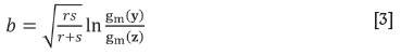
where g_m(.) is the geometric mean of the arguments; y and z are groups of parts determined in the SBP; and r and s are the number of parts in y and z, respectively. Balances are scale-invariant quantities. They are also orthogonal log-contrasts (Aitchison, 2003, p. 85). As a consequence, computation of balances does not change with the units of the parts in the composition, or whether they are closed or not. This is important for applications, like the one presented in this contribution, where only some parts of the whole composition not exactly adding to a constant are modelled.

The ilr transformation and its inverse, plus a basis constructed using a SBP, have compact expressions useful for computation. Consider a (D -1,D)-matrix Θ, with entries θ_ijwhich can take the values +1, -1, 0. Each row of Θ encodes one partition of the SBP. For the i-th row, θ_ij = +1 points out that x_jbelongs to the group of parts G_i+; similarly, θ_ij= -1 indicates that x_jis in the group of parts G_i-; θ_ij= 0, meaning that x_jis not involved in the i-th partition. From the SBP code Θ, the so-called contrast (D-1,D)-matrix Ψ is built up (Egozcue and Pawlowsky-Glahn, 2005, 2006; Tolosana-Delgado et al., 2008; Egozcue et al., 2011). If θ_ij= 0, the corresponding entry of Ψ, ψ_ij , is also null. For θ_ij= +1 and θ_ij= -1 the values are, respectively:

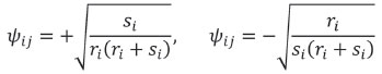
where r_i, s_i are the number of +1 and -1 in the i-th row of Θ. The ilr transformation and its inverse are

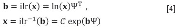
where x, b are row-vectors, with D -1 and D components, respectively; the logarithm, ln, and the exponential, exp, operate component-wise; and (·)^T denotes matrix transposition.

Orthogonal projections for compositions

Projections are the main tool of dimension reduction in data analysis. Dimension reduction of compositions is not an exception. Orthogonal projections make sure that distances between compositions are shorter in the projection than in the original D components. Therefore, projections for dimension reduction should be orthogonal (Egozcue and Pawlowsky-Glahn, 2005). The simplest case consists in using only some parts of a composition. This is an orthogonal projection on a subcomposition. However, there are other possible projections that do not correspond to this elementary case. In general, projections are better described in terms of coordinates and, particularly, using balances built up from a SBP.

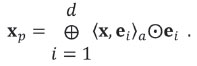
The rationale of a generic, orthogonal, projection is as follows. A subspace of the simplex, , is defined by a set of d orthogonal, unitary, compositions e₁, e₂,..., e_d, d ≤ D-1, which constitute a basis of the subspace. The projection of x ∈ S^Dinto the d-dimensional subspace is determined by the inner product 〈x, e_i〉_α>, i = 1,2,...,d. The orthogonal projection of x on the subspace is

The basis of the subspace , e₁, e₂,..., e_d, can be extended to a basis of S^D, by adding a set of unitary compositions, e_d+1e_d+2...,e_d-1such that they are mutually orthogonal, and orthogonal to the basis of the subspace. The coordinates of x in this basis are b_i = 〈x, e_i〉_α>, i = 1,2,..., D-l. Evidently, projecting x on the subspace reduces to making b_i= 0 for i = d +1, d +2,..., D-1. In order to express the projection in the simplex, the ilr-inverse transformation (Equation [4]) is used. Denote the original ilr-coordinates, arranged in the D-1-vector by b, and the ilr-coordinates after the projection, b_p. If Ψ is the contrast matrix corresponding to the basis e₁, e₂,..., e_D-1, the projected composition x_p is obtained as

The assumption is that there is a reference subcomposition of interest and the projection to be carried out should retain all relative proportions contained in the reference subcomposition. The situation studied herein is a projection on a subspace including the reference subcomposition and other supplementary data. In general, any orthogonal projection of compositions suppresses the units in which the original composition was presented. There are scenarios in which it is worthwhile to have the projection using the original units. Consequently, it is worthwhile to study how to recover original units after an orthogonal projection, which involves modelling some kind of total and the corresponding projection.

After expressing a composition x ∈ S^D in D − 1 coordinates, ignoring the rest, is equivalent to an orthogonal projection of x,thus reducing the dimensionality of the analysis. The choice of an orthogonal projection depends on the problem to be studied, and on the interpretability of the coordinates. The use of balances coming from a SBP is encouraged, as they can lead to easily interpretable coordinates.

Orthogonal projection on a subcomposition using balances

In practice, the most frequent orthogonal projection is on the subspace of a given reference subcomposition. Suppose that this subcomposition is [x₁,x₂,..., x_d+i]· The subcomposition is supposed to be made up of the first d +1 parts of x. There is no loss of generality in this assumption, as the parts in xcan always be reordered by a convenient permutation. An orthonormal basis for the subcomposition x_s is readily built up using a SBP. Let b₁ be the balance (coordinate) comparing the subcomposition x_s to the other parts in the composition, and b_i, i = 2,...,d, be the balances (coordinates) corresponding to x_s. The SBP of x_s can easily be extended to the original composition. Regardless of the extension of the SBP, balances b_i, i = 2,...,d, of x are equal to those corresponding to x_s because balances are not affected by the closure applied to compute x_s. Thus, projecting on a subcomposition is equivalent to keeping the balances b₂,b₃,..., b_d and setting the remaining balances to zero, i.e. b₁, = 0 and b_d+1= 0,...,b_D-1= 0, to form the vector of b_p= 0. Table I illustrates how this projection works for an example of D = 6 parts with d = 1, i.e. projection on a reference subcomposition of two parts. The projection on the reference subcomposition, [x_1,x₂] is obtained by setting b₁ = 0 and b_j = 0 for j = 3, 4, 5. From b_p the projected composition is obtained using ilr-inverse in Equation [5] (Egozcue and Pawlowsky-Glahn, 2005).

 

 

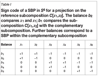
The strategy of projecting the reference subcomposition may be not appropriate if some property from the complementary subcomposition is relevant and needs to be preserved. The obvious way of doing this consists in using the D-1 coordinates corresponding to the original composition x with no reduction of dimension at all. An intermediate possibility is considering both the coordinates of the reference subcomposition and one or more balances including parts in the complementary subcomposition. In the present example, we have taken only two balances, b1 and b₂,to keep the presentation simple. Balance b₂ corresponds to the reference subcomposition [x₁x₂], and balance b₁compares [x₁,x₂] vs. [x₃,x₄,..., x₆]; although filtering out details within each group, the balance b₁ is an interesting candidate to be preserved in the projection. Following the example in Table I, using only b₁and b₂ is equivalent to an orthogonal projection from a five-dimensional space, , into a subspace of dimension 2, which is a substantial dimension reduction.

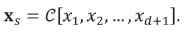
The reference subcomposition is

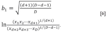
Using an SBP within x_s the balances b₂,b₃,..., b_d are readily obtained. Also b₁ corresponds to the partition of x into the reference subcomposition and its complement, and its expression is

The SBP of x is extended with an SBP of the complementary subcomposition, as illustrated with the example in Table I.

A useful projection is to preserve the values of the balances corresponding to the reference subcomposition b₂,b₃,..., b_d and b₁; other balances are set to zero. Denoting by b_p these projected balances, the ilr-inverse (Equation [5]) provides the projection (Egozcue and Pawlowsky-Glahn, 2005):

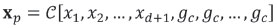
where g_c is the geometric mean of parts within the complement of the reference sub-composition; this geometric mean is repeated D - d -1 times to have the D parts. The geometric mean g_c is a summary of the data within the complementary subcomposition. Moreover, , but it spans only a (d + 1)-dimensional subspace. The vector x_p can be represented by its balances b_p= [b₁,b₂,..., b_d,0,...,0] where the reduction of dimension appears effective.

Other balances amongst b_d+1,b_d+2,..., b_D-1 can also be preserved, producing orthogonal projections on subspaces of larger dimension. The choice of these projections should be related with the nature of the problem to be solved, and with the relevance of the balances preserved. The proposed selection of specific balances is here related to the characteristics of the orthogonal projection, but subsequent operations and modelling could be performed using any set of coordinates.

Results in the original units after a projection

Inverse transformed values are parts adding to 1 . When the parts add to a different constant, such as concentrations adding to a million, the required scaling is trivial: all parts need to be multiplied by the constant. In cases, such as molar concentrations or mg/ℓ, the backtransformation to the original units requires a more demanding scaling. Suppose that a D-part composition x is expressed in some meaningful units. For instance, in percentages, ppm, ppb, mg/ℓ or the like. Frequently, the fill-up component is omitted, and x appears as a non-closed vector. A closure of x causes the change of the original units. Also, after any orthogonal projection, these units are lost. In the simplest case, projection on a reference subcomposition, the result will be expressed as proportions within the subcomposition as an effect of the closure of the subcomposition. In some cases, the analyst can be interested in having the final results in the original units after projections such as those presented above. If the original composition is large, the interest might be in obtaining the parts in the reference subcomposition in the original units. However, such a demand cannot be satisfied in a strictly compositional framework. A kind of total needs to be known. Totals can be defined in a variety of ways (Pawlowsky-Glahn et al., 2013 and 2014), but some of them are quite intuitive - for instance, the sum of parts in a given subcomposition, or even a single part, using the original units. In general, totals, denoted t, arepositive quantities with sample space or a two-part simplex . Following the principle of working in coordinates (Pawlowsky-Glahn and Egozcue, 2001; Mateu-Figueras et cel., 2011) the total is modelled by its only coordinate in ,or in closed to a constant K_t. In the first case the coordinate is In t; in the case of , the coordinate is proportional to ln (t/( K_t-t)) (the logit transformation of t). Here, these coordinates are denoted generically by φ(t).

The following procedure is aimed at obtaining the original units for the parts in the reference subcomposition. We assume that the projection is defined by the balances b₂,b₃,..., b_d, of the subcomposition, plus b₁ as defined previously in Equation [6]. For this kind of projection, the total, t = x₁+ ... + x_d+1, expressed in the original units, is a useful choice, and will be used from now on. The total t can be obtained from its coordinate using φ^-1, i.e. if φ(t) = ln t, φ-1 is the exponential function; if τ= φ(t) = ln (t/((K_t-t))), then t = φ^-1 (τ) = exp(τ)/[1 +exp(τ)]. The procedure to have the projected parts in the original units has three steps, with the two first ones corresponding to the projection:

1 Find the balance-coordinates of x. Set some of them to zero to perform the desired projection, thus obtaining the projected balances b_p

2. Obtain x_p,closed to some constant κ, applying the inverse ilr-transformation to the projected balances b_p

3. Re-scale x_p to the original units, using the total t, to finally obtain the parts in x_s in the original units.

The two first steps have been described in the previous section. The third step is the calculation necessary to have the concentrations in the original units in x_p. The vector containing the projected composition, scaled to the original units, is

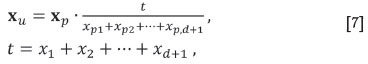
where the role of the total t appears clearly. The x_u is a closed composition when considering the original D-parts plus the fill-up value; but the first parts x_u1,...,x_u,d+1, corresponding to the reference subcomposition do not appear closed as a subcomposition. On the other hand, the closure constant κdoes not appear explicitly in the scaling, as it cancels out when dividing by Σ_ix_pi.

Cokriging

In our approach, the primary result of a spatial-compositional analysis is a set of interpolated maps of balances. The interpretation of these maps depends on the definition of the particular balances chosen by the analyst. However, the standard practice may require the analyst to generate a map of the concentration of a single part using the original units, e.g. in the following section, the illustrative example uses milligrams per litre. Then, a procedure to translate the results, expressed in balances, into a single element concentration is also required.

Cokriging is a multivariate method for the simultaneous interpolation of several regionalized variables. Obtaining interpolated maps of D ‒ 1 balances using cokriging may be a hard task if D is a moderate to large number. To avoid such a challenging task, attention can be centered in a reference subcomposition containing d + 1 parts. Projections presented previously reduce the number of variables to be cokriged in a consistent way to d + 1 balances.

As pointed out in Myers (1983), cokriging should be performed before any projection or dimensional reduction of the data. Here we confront the tradeoff between the simplification of cokriging and the loss of measurement units - μg/ℓin our case ‒ caused by the projection of the compositional vector. In order to mitigate this loss, the alternative projection is preferred. For the sake of simplicity, only d + 1 balances will be cokriged. Additionally, interpolated values of the parts in the reference subcomposition in the original units are also required. As stated in the previous section, a total is also needed, and its coordinate φ(t) should also be cokriged with the mentioned d +1 balances. Therefore, cokriging involves d + 2 variables.

The balances b₁,b₂,...,b_d+1 and φ(t) are transformed variables which have no support restrictions: they can span the whole real line, and they are no longer compositional or positive variables. Ratios of parts of compositions are frequently positively skewed, thus approximating lognormal distributions. These distributions approach normal distributions when log-transformed (Mateu-Figueras et al., 2011). Hence, standard multivariate techniques can be applied to these log-transformations. In particular, cokriging can be applied, and the properties of cokriging properly hold: best (minimum variance) linear unbiased estimator.

To perform cokriging of the vector of these d + 2 variables, we use a matrix formulation of cokriging (Myers, 1982). Some advantages are:

►The components of the estimation vector are estimated simultaneously instead of repeating d + 2 times the undersampled formulation of cokriging, where the roles of primary and secondary variables are interchanged

►The full variance-covariance of the estimates is provided, while only the cokriging estimation variance is obtained when each variable is estimated separately

►Myers (1982) concludes that matrix formulation is computationally advantageous and the cross-semivariogram model is clearer.

For clarity of notation in the remainder of this section, non-random (column) vectors are denoted in lowercase and boldface, and matrices are presented in boldface capitals. Random variables are presented in capitals, and boldface if they form a random (column) vector. Let Z = (Z₁Z₂,...,Z_m) denote the vector of second order stationary random functions modelling the variables of concern; here they are (b₁,b₂,...,b_d+1,φ(t)). The random vector Z is observed in the set of n data locations u_k, k =1, 2,...,n, normally expressed in coordinates as northing and easting in the case of a bidimensional spatial domain. The goal of cokriging is to estimate Z at a location u₀, Z( u₀), using the linear estimator

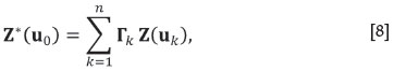
where Γ_k is an (m, m)-matrix of weights. The weights Γ_k are obtained by minimizing an estimation variance, conditional to Z*(u₀) being an unbiased estimator of the mean value of Z(u₀). A sufficient condition for Z*(u₀)to be unbiased is that

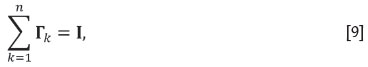
(Myers, 1982), where I is the (m, m)-identity matrix. Although there are different ways of defining the estimation variance in the multivariate estimation case, the form

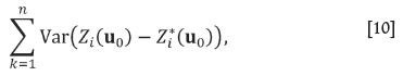
is computationally advantageous. Minimization of the estimation variance (Equation [10]), subject to the unbiasedness condition [9], determines the weights, Γ_k, by solving the cokriging system of equations

(Myers, 1982), where the number of equations is m· (n + +1) and

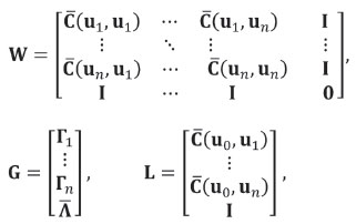
with an estimator of the covariance matrix of Z(u_i)and Z(uj), and an (m, m)-matrix of Lagrange multipliers. The variance-covariance matrix of the estimator Z*(u₀)is

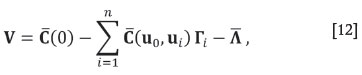
(Myers, 1982), where which does not depend on u_i under second order stationarity of Z.

The cokriging estimator Z^*(u₀) is a linear combination of the observations Z(u_k) whenever the observed variables are real. However, if Z is taken as a raw composition, several disappointing consequences follow (Pawlowsky, 1984). The first one is that Z*(u₀) is no longer a linear estimator, as the linear combination in Equation [8] becomes nonlinear in the simplex, (see section on Aitchison geometry for compositional data) and ill-defined, as the non-convex combination of compositions is not assured to be a composition (Pawlowsky-Glahn et al., 1993). A second issue of concern is that the unbiasedness property is lost because the centre of a random composition is not the mean when the composition is taken as a real vector (Aitchison, 1986; Pawlowsky-Glahn and Egozcue, 2001, 2002). A third pitfall is that all covariance matrices appearing in the cokriging equations ([11]-[12]) are spurious (Aitchison, 1986; Egozcue and Pawlowsky-Glahn, 2011; Pawlowsky, 1984).

 

Application: As and Fe in the groundwaters of Bangladesh

Available data

A well-known public-domain data-set is used to illustrate the above methodology: groundwater geochemical analysis conducted in the late 1990s in Bangladesh jointly by the local Department of Public Health Engineering and the British Geological Survey (2001a, b). The main objective of this exercise is to illustrate the adequate mapping of compositional data in general, not touching on other important and related subjects such as the genesis of the concentrations and the public health implications. The Bangladesh raw data require some pre-processing to address the following issues:

(a) There are indications in the British Geological Survey (2001a) report, supported also by Yu et al. (2003), that there is a systematic tendency of the As concentration to decrease with depth. This fact implies that proper modelling of the entire data-set requires a three-dimensional modelling. The simpler two-dimensional mapping of our interest thus requires the subdivision of the complex system of aquifers and aquitards into units without significant vertical fluctuations in concentration. Inspection of the data and the geology suggested that the aquifer between 7-41 m was sufficiently homogeneous for a two-dimensional modelling. This is the subject of the present application

(b) Another issue is that some of the values are below detection limit, that is, values greater than zero but small enough to be below the analytical precision of the laboratory. The detection limit for As is 0.5 μg/ℓ and 0.005 mg/ℓ for Fe. All data values below detection limits were replaced by an imputed value using the methodology described in Olea (2008)

(c) Four wells were discarded because all values were below detection limit, an unlikely situation in nature, which prompted the authors to suspect errors in the collection or processing of the specimens.

The original data-set consisted of 3416 records, each one containing the concentration of 20 solutes in water (parts) in milligrams per litre. Of the 20 parts analysed in the survey, Co, Cr, Li, V, Cu, and Zn were not considered, as they present serious problems related to values below detection limits and to rounding in the measurement process. The arsenic values were an exception in the sense that they were reported in micrograms per litre, but were changed to milligrams per litre for the purpose of modelling. The reader can visit the Internet to view maps posting the data (British Geological Survey, 2001a).

Here, only the set of solutes (As, Al, B, Ba, Ca, Fe, K, Mg, Mn, Na, P, Si, SO₄, Sr) is considered. A data-set consisting of 14 solutes and 2096 data locations was thus retained for further analysis.

Modelling

In the present development, available data corresponds to D = 14 parts of a larger composition in milligrams per litre. An analysis could be performed defining a fill-up value to the total given by the units of measurement. This method would require the analyst to know the density of water and the fill-up variable would essentially be water, for example, as done in Otero et al. (2005). Here, the fill-up part is ignored and only data in x∈ S 14 is modelled. The subcomposition (As, Fe) is taken as the reference subcomposition. The available compositions at the observation points are projected following the approach developed previously, i.e. d = 1.

According to the emphasis by the British Geological Survey (2001a), interest is centred on As and Fe; therefore, the SBP was defined in a way that the first balance, b₁, reflects the relation of (As, Fe) versus the rest of parts, and the second balance, b₂, the relation of (As vs Fe). Following Equation [3], they are computed as:

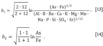
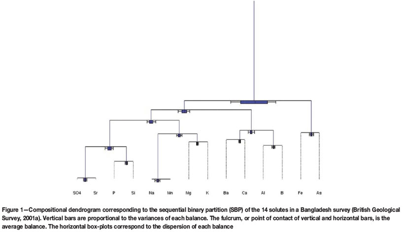
The remaining D - 2 = 12 balances were defined without specific geological criteria. The following analysis does not depend on the choice of these balances. The SBP used is graphically displayed as the compositional dendrogram (Thió-Henestrosa et al., 2008; Pawlowsky-Glahn and Egozcue, 2011) shown in Figure 1, obtained with the package CoDaPack (Comas-Cufí and Thió-Henestrosa, 2011).

The uppermost vertical bar, corresponding to the partition (As, Fe) versus the rest of parts, is the largest because the variance of b₁ is the largest one. It is, in fact, 5.4805, while b₂ has a variance of 1 .7401, which is the second largest variance. Balances b₃,b₄,...,b₁₃ are not necessary in the following analysis, and are not included in the cokriging system of equations.

Following the approach outlined previously, the total considered for having the results in the same original units is t = As + Fe mg/ℓ. The number of variables to be cokriged is then d +2 = 3, i.e. b₁, b₂, φ(t). The balances b₁ and b₂ are dimensionless, as in Equations [13] and [14] units disappear, while the units of t are the original milligrams per litre. The total variable t has compositional character because it is the ratio t over the total mass (solute and water) per litre. Frequently, the total mass, taken equal to k_t = 10⁶ mg/ℓ and (t,10⁶-t), is a composition in . In that case, the coordinate φ(t) would be the logit transform of t, as mentioned previously. However, taking k_t = 10⁶ mg/ℓ is inadequate, as it ignores the mass of solute (Otero et al, 2005). The alternative of considering t as a variable in ℜ₊ has been chosen and, consequently, φ(t) = In(t) is considered as the corresponding coordinate to be used in the cokriging modeling.

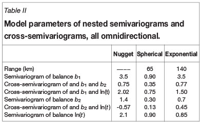
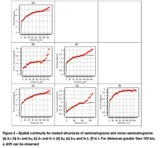
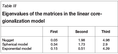
The parameters of semivariograms and cross-semivariograms used for cokriging are given in Table II, and are displayed in Figure 2. Table III gives the eigenvalues for the coefficient matrices in the linear coregionalization model used in the inference of spatial correlation.

 

 

 

 

 

 

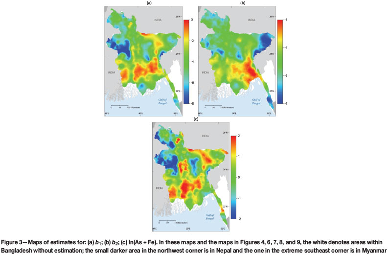
The study area was tessellated into a grid of locations with a spacing of 1 km comprising 460 columns and 660 rows with 123 079 of the locations within the borders of Bangladesh, covering the country with reasonable resolution. Cokriging was applied using the linear coregionalization models of Table II. The estimated maps of b₁, b₂, and ln (t) are shown in Figure 3. Maps (a) and (b) in Figure 3 contain the estimates balances after the projection of the whole composition and the corresponding cokriging. However, obtaining the results in the same original units (OU) of arsenic and iron is performed using Equations [5] and [7], which requires the cokriging results shown in map (c) of Figure 3 corresponding to natural logarithm of the sum of the two elements, both in the original units.

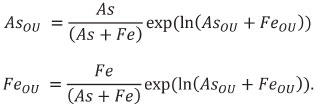
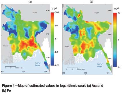
Figure 4 shows the interpolation of both elements in their original units mg/ℓ. Despite its relevance, concentrations of arsenic are quite low relative to the other elements in the survey. So, for display, all values were multiplied by 1000 to change units to μg/ℓ , the standard form of reporting arsenic concentrations in hydrochemistry. These maps show that the compositional techniques are able to perform orthogonal projections to reduce the dimension of cokriging, and to express the results in the traditional form of maps of a single solute in the original units mg/ℓ.

 

 

Uncertainty evaluation of As and Fe

Equation [12] is the variance-covariance matrix of the estimators. If the analyst is willing to assume multinormality of errors, the results can be used to assess uncertainty in the modelling. In particular, three measures have been computed: (a) the probability that As and Fe exceed a given threshold of concentration in milligrams per litre; (b) confidence intervals on As and Fe; and (c) validation of the coverage of the computed confidence intervals.

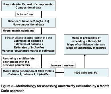
The scheme of the general procedure is shown in Figure 5. For each point in the interpolation grid, 1000 joint replications of (b₁, b₂, ln t) have been generated using the Cholesky method (Davis, 1987), following a multivariate normal distribution with a mean equal to the three estimated fields (Figure 3) and covariance V (see third step in the work-flow, Figure 5). The simulation step corresponds to the fourth step in Figure 5. The next step is the reconstruction of the concentrations of As and Fe from the simulated triplets (b₁, b₂, ln t). It consists of applying the ilr-inverse transformation to (b₁, b₂) (Equation [5]) to produce the closed reference subcomposition (As, Fe). Then (fifth step in the work-flow, Figure 5), using the simulated value of ln (t) = ln(As+Fe), Equation [7] allows the analyst to obtain the subcomposition in the original units (milligrams per litre).

 

 

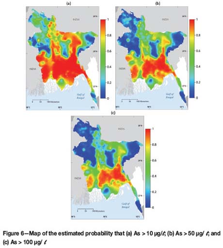
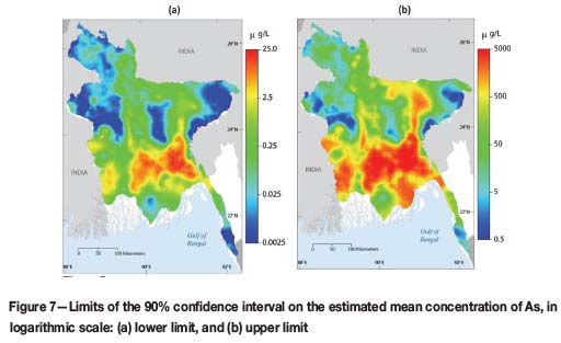
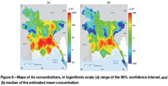
The results from simulation are presented in several maps. Figure 6 shows the probability of the content of As exceeding 10, 50, and 100 μg/ℓ. The first limit of 10 μg/ℓ is the drinking water upper limit established by the World Health Service (WHS); the limit of 50 μg/ℓ is the limit used in Bangladesh, and 100 μg/ℓ is an arbitrary threshold that is 10 times the limit of the WHS and double the Bangladesh recommendation. The maps in Figure 6 show a large probability of exceeding the three limits of interest in more than the 50% of the area of Bangladesh. Other statistics that have been computed are the lower and upper limits of the 90% confidence interval on the mean value of As, the width of the interval (upper limit minus lower limit), as well as the median and standard deviation of the Monte Carlo distribution of As (Figures 7 and 8, respectively).

 

 

 

 

 

 

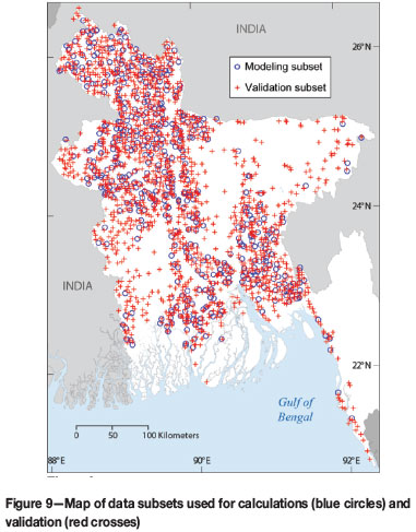
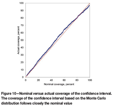
In order to proceed to a validation of the model, the data-set has been divided into two groups (Figure 9): a calibration set (519 values) and a validation set (1577 values). For each location in the validation set, the mean value of the triplet (b₁, b₂, ln t) is predicted from the points in the calibration set using the semivariograms (Table II); also the variance-covariance matrix V is taken from the global analysis. Then, a multivariate normal with these parameters is simulated 1000 times at each validation point. It produces triplets (b₁, b₂, ln t), which can be used to obtain simulated values of As and Fe. The probabilistic meaning of the α% Monte Carlo confidence intervals have been validated exhaustively by varying αfrom 0.01 to 0.99 and calculating the actual coverage by using the validation set from the previous validation exercise. The results are shown in Figure 10, where the nominal coverage is compared with the actual coverage. The results follow closely the 1:1 line, indicating the good agreement between nominal and actual coverage. The result confirms that, at least for the As concentration in Bangladesh, the combined use of balances and assumption of multinormality of errors is adequate. Considering that the modelling is independent from the physical nature of the analysed system, the modelling should work correctly for any other spatial compositional data.

 

 

 

 

Discussion in terms of practical results

In a strict sense, our practical results are not comparable to any of those from previous studies using the same Bangladesh data, because of our decision to limit our modelling within the depth range of 7-41 m below surface and our imputation of values below the detection limits. The original study set the cut-off at 150 m (British Geological Survey, 2001a; Gaus et al., 2003), a practice followed by most other authors mentioned toward the end of the Introduction. Among the exceptions, Shamsudduha (2007) restricted his study to depths up to 25 m. Hossain et al. (2007) set the second shallowest cut-off behind ours at 75 m. On the less consequential issue of replacement of values below detection limit, again most authors followed the lead of the original British Geological Survey Report (2001a) of doing nothing - treating the detection limits as actual measurements - or replacing them by half the value of the detection limit. Instead, we used a method to extrapolate the probability distribution of values below detection limit (Olea, 2008). Hossain et al. (2007) unilaterally assigned the value 1 part per billion (ppb) to all values below detection limit, without noting or caring that 1 ppb is different from 1 μg/ℓ.

Despite working with different subsets of the same original data, maps of expected arsenic concentrations produced applying different methods are remarkably similar, as it is the case, for example, of our Figure 4a and the equivalent Figure 6.4 in the original study (British Geological Survey, 2001a, vol. 2, p. 83). Shamsudduha (2007) addresses the issue of lack of sensitivity to estimation methods by applying six different methods to the same data, including ordinary kriging without any transformation of the data, which has the potential of producing negative concentrations. This unacceptable inconsistency illustrates the potential danger of avoiding the use of compositional methods because, while non-compositional modelling appears to provide reasonable results most of the time, results may not always be coherent and optimal. At least at the present time, exact number and location of problematic estimates are impossible to predict. Unfortunately, there are no analytical expressions available to assess differences in results between compositional and noncompositional approaches. Discussion of methodological assumptions and comparison of numerical examples remain as the only approaches to evaluate alternative methods.

In addition to the desire to have optimal estimates, the main interest in applying stochastic methods to complex systems is to obtain measures of uncertainty associated with the modelling. There are several ways to display such uncertainty, ways that are not always easy to compare, for example, magnitude of potential errors or length of confidence intervals. Hossain et al. (2007), applying ordinary kriging to a logarithmic transformation of the data, made a cross-validation by evenly splitting at random the data into values used in the modelling and control points to compare results. For a 10 μg/ℓ threshold, they found that only 72.2% of the wells were correctly predicted to be safe. Serre et al. (2003) used a Bayesian maximum entropy approach to prepare two traditional maps: one for the estimate and another for their standard errors. Relative to our results, their standard errors, on average, are one order of magnitude smaller. Maps of probability of exceedance above selected thresholds are one of the most useful displays in geochemistry, a practice that had been abandoned by all authors of publications after the release of the British Geological Survey (2001a) report. The original study contains probabilities of exceedance for 5, 10, 50, and 150μg/ℓ based on disjunctive kriging of logarithmic transformations (British Geological Survey, 2001a, vol. 2, p. 169). Our Figures 6a and 6b are the same type of maps for the second (As μg/ℓ) and third thresholds (As μg/ℓ). Our probabilities are significantly higher than those in the original report, suggesting that avoiding the balance approach to mapping compositional data seems to produce low probabilities of exceedance, which in cases of toxic elements in groundwater translates into false negatives ‒ a dangerous situation in which the population is given assurance of safe drinking water when it may not, in fact, be safe. Our unique validation of confidence intervals (Figure 10) gives us assurance that our results are not an exaggerated claim about the possible existence of high concentrations, but a closer approximation to reality.

 

Conclusions

Compositions are a special type of data about relative proportions of variables in a system. All the parts of a composition, if present, are non-negative. Frequently, they are reported in such a way that they add to a constant to insure that data can be compared independently of the physical size of the specimens. In this case, the data values are in a simplex; they are thus constrained and do not vary over the whole real space. Consequently, statistical methods valid for data varying over the whole real space are not directly applicable to compositional data in a simplex, including cokriging.

Application of cokriging to compositional data requires as a minimum a different representation of the data, i.e. a representation in coordinates. This transformation moves the compositional data from the simplex to the whole real space. General purpose transformations, devised for other, unconstrained, regionalized variables, are unsatisfactory for compositional data because they do not properly handle the relative proportions carried by the data. The ilr transformation attains this goal, in particular because it is scale-invariant and subcompositionally coherent. Other transformations commonly used in compositional data analysis, such as the alr (additive logratio) and the clr (centered logratio), have not been considered. The alr leads to an oblique basis, distorting the measures of error like the kriging variance, when they are used as being orthonormal. The clr leads to a generating system with singular covariance matrices. Moreover, the use of ilr transformations to obtain coordinates makes the work with orthogonal projections easy, thus providing a way of supervised dimension reduction. Orthogonal projections in the simplex (e.g. on a subcomposition or defined through balances) allows generation of results in the same units as the input data, even if the sum of all parts do not add to a constant provided that some type of total in the original units is available.

Cokriging is the best multivariate method to use in producing estimates of compositional data at locations away for observation sites. In combination with Monte Carlo methods, under an assumption of multinormality of the balances, it is possible to assess the uncertainty of the estimators. Some theoretical advantages of the approach are:

(a) Scale-invariance and subcompositional coherence

(b) Controlled dimension reduction using orthogonal projections

(c) The possibility of having the results in the same original units

(d) Modelling using balances can result in estimation errors whose distribution can be assumed to be approximately multinormal in the transformed space

(e) Using Monte Carlo simulation to expand the cokriging results, it is possible to assess the uncertainty of the cokriging modelling.

Good conformance in confidence intervals indicates that the modelling in general, and the multinormality assumption in particular, are acceptable in this case. We have revisited the mapping of a hydrochemical survey from Bangladesh. We and the British Geological Survey applied different transformations and estimation methods. Indications are that the discrepancies are more significant in terms of assessing uncertainty than in terms of mapping expected values. At least in this comparative evaluation, the original study obtained lower probabilities of exceedance, more likely because of lack of adequacy of the transformations than because of the differences in estimation methods.

 

Acknowledgments

We are grateful to Raimon-Tolosana-Delgado (Helmholtz-Zentrum Dresden-Rossendorf, Germany), James Coleman (US Geological Survey), Michael Zientek (US Geological Survey) and an anonymous reviewer appointed by the journal for critically reviewing earlier versions of this paper. Eric Morrissey (US Geological Survey) and Christopher Garrity (US Geological Survey) helped us in the annotation of the maps.

This research has been partly supported by the Spanish Ministry of Economy and Competitiveness under the project METRICS (Ref. MTM2012-33236); and by the Agencia de Gestió d'Ajuts Universitaris i de Recerca of the Generalitat de Catalunya under project Ref: 2009SGR424.

Any use of trade, firm, or product names is for descriptive purposes only and does not imply endorsement by the US Government.

 

References

Aitchison, J. 1982. The statistical analysis of compositional data (with discussion). Journal of the Royal Statistical Society, Series B (Statistical Methodology) vol. 44, no. 2. pp. 139-177.         [ Links ]

Aitchison, J. 1986. The Statistical Analysis of Compositional Data. Monographs on Statistics and Applied Probability. Chapman & Hall, London (UK). (Reprinted in 2003 with additional material by The Blackburn Press). 416 pp.         [ Links ]

Aitchison, J. 2003. The Statistical Analysis of Compositional Data. The Blackburn Press, Caldwell, NJ. 435 pp.         [ Links ]

Anwar, A. and Kawonine, N. 2012. Characterization of arsenic contamination in groundwater by statistical methods. International Journal of Global Environmental Issues, vol. 12, no. 2-4. pp. 302-317.         [ Links ]

Barceló-Vidal, C., Martín-Fernández, J.A., and Pawlowsky-Glahn, V. 2001. Mathematical foundations of compositional data analysis. Proceedings of IAAMG'01 - The Sixth Annual Conference of the International Association for Mathematical Geology. Ross, G. (ed.), pp. 1-20.         [ Links ]

Billheimer, D., Guttorp, P., and Fagan, W. 2001. Statistical interpretation of species composition. Journal of the American Statistical Association, vol. 96, no. 456. pp. 1205-1214.         [ Links ]

British Geological Survey. 2001a. Arsenic contamination of groundwater in Bangladesh. Technical report, BGS, Department of Public Health Engineering (Bangladesh). 630 pp. (Report WC/00/019). http://www.bgs.ac.uk/arsenic/Bangladesh/        [ Links ]

British Geological Survey. 2001b. Arsenic contamination of groundwater in Bangladesh: data. Technical report, BGS, DPHE/BGS National Hydrochemical Survey, 1 Excel spreadsheet. http://www.bgs.ac.uk/research/groundwater/health/arsenic/Bangladesh/data.html)        [ Links ]

Chayes, F. 1960. On correlation between variables of constant sum. Journal of Geophysical Research, vol. 65, no. 12. pp. 4185-4193.         [ Links ]

Chayes, F. 1962. Numerical correlation and petrographic variation. Journal of Geology, vol. 70, no. 4. pp. 440-452.         [ Links ]

Chayes, F. 1971 . Ratio Correlation. University of Chicago Press, Chicago, IL. 99 pp.         [ Links ]

Chayes, F. 1975. A priori and experimental approximation of simple ratio correlations. Concepts in Geostatistics. McCammon, R.B. (ed.). Springer Verlag, New York. pp. 106-137.         [ Links ]

Chayes, F. 1983. Detecting nonrandom associations between proportions by tests of remaining-space variables. Mathematical Geology, vol. 15, no. 1 . pp. 197-206.         [ Links ]

Chowdhury, M., Alouani, A., and Hossain, F. 2010. Comparison of ordinary kriging and artificial neural network for spatial mapping of arsenic contamination of groundwater. Stochastic Environmental Research and Risk Assessment, vol. 24, no. 1. pp. 1-7.         [ Links ]

Comas-Cufí, M. and Thio-Henestrosa, S. 2011. CoDaPack 2.0: a stand-alone, multi-platform compositional software. CoDaWork'11: Proceedings of the 4th International Workshop on Compositional Data Analysis, Sant Feliu de Guíxols, Girona, Spain. Egozcue, J.J., Tolosana-Delgado, R., and Ortego, M. (eds.). International Center for Numerical Methods in Engineering. Barcelona, Spain.         [ Links ]

Davis, M. 1987. Production of conditional simulations via the LU triangular decomposition of the covariance matrix. Mathematical Geology, vol. 19, no. 2. pp. 91-98.         [ Links ]

Egozcue, J.J., Barceló-Vidal, C., Martín-Fernández, J.A., Jarauta-Br Agulat, E., Díaz-Barrero, J.L., and Mateu-Figueras, G. 2011. Elements of simplicial linear algebra and geometry. Compositional Data Analysis: Theory and Applications. Pawlowsky-Glahn, V. and Buccianti A. (eds.). Wiley, Chichester, UK. 378 pp.         [ Links ]

Egozcue, J. J. and Pawlowsky-Glahn, V. 2005. Groups of parts and their balances in compositional data analysis. Mathematical Geology, vol. 37, no. 7. pp. 795-828.         [ Links ]

Egozcue, J. J. and Pawlowsky-Glahn, V. 2006. Simplicial geometry for compositional data. Compositional Data Analysis in the Geosciences: From Theory to Practice. Buccianti, A., Mateu-Figueras, G., and Pawlowsky-Glahn, V. (eds). Volume 264 of Special Publications. Geological Society, London. 212 pp.         [ Links ]

Egozcue, J. J. and Pawlowsky-Glahn, V. 2011. Basic concepts and procedures. Compositional Data Analysis: Theory and Applications. Pawlowsky-Glahn, V. and Buccianti, A. (eds.). Wiley, Chichester, UK. 378 pp.         [ Links ]

Gaus, I., KinniburghI, D., Talbot, J., and Webster, R. 2003. Geostatistical analysis of arsenic concentration in groundwater in Bangladesh using disjunctive kriging. Environmental Geology, vol. 44, no. 8. pp. 939-948.         [ Links ]

Hassan, M. and Atkins, P. 2011. Application of geostatistics with indicator kriging for analyzing spatial variability of groundwater arsenic concentrations in southwest Bangladesh. Journal of Environmental Science and Health, Part A, vol. 46, no. 11. pp. 1185-1196.         [ Links ]

Hossain, F., Hill, J., and Bagtzoglou, A. 2007. Geostatistically based management of arsenic contaminated ground water in shallow wells of Bangladesh. Water Resources Management, vol. 21, no. 7. pp. 1245-1261.         [ Links ]

Hossain, F. and Sivakumar, B. 2006. Spatial pattern of arsenic contamination in shallow wells of Bangladesh: regional geology and nonlinear dynamics. Stochastic Environmental Research and Risk Assessment, vol. 20, no. 1-2. pp. 66-76.         [ Links ]

Hossain, M. and Piantanakulchai, M. 2013. Groundwater arsenic contamination risk prediction using GIS and classification tree method. Engineering Geology, vol. 156. pp. 37-45.         [ Links ]

Martín-Fernández, J.A., Barceló-Vidal, C., and Pawlowsky-Glahn, V. 1998. Measures of difference for compositional data and hierarchical clustering methods. Proceedings of IAMG'98 - The Fourth Annual Conference of the International Association for Mathematical Geology. Buccianti, A., Nardi, G., and Potenza, R. (eds.). De Frede Editore, Naples. pp. 526-531.         [ Links ]

Mateu-Figueras, G., Pawlowsky-Glahn, V., and Egozcue, J.J. 2011. The principle of working on coordinates. Compositional Data Analysis: Theory and Applications. Pawlowsky-Glahn, V. and Buccianti, A. (eds.). Wiley, Chichester, UK. pp. 31-42.         [ Links ]

Myers, D.E. 1982. Matrix formulation of co-kriging. Mathematical Geology, vol. 14, no. 3. pp.249-257.         [ Links ]

Myers, D.E. 1983. Estimation of linear combinations and co-kriging. Mathematical Geology, vol. 15, no. 5. pp. 633-637.         [ Links ]

Olea, R. 2008. Inference of distributional parameters of compositional samples containing nondetects. Proceedings of CoDaWork'08, The 3rd Compositional Data Analysis Workshop, Universitat de Girona, Girona, Spain. Daunis-i Estadella, J. and Martín-Fernández, J.E. (eds.). http://dugi-doc.udg.edu/handle/10256/708 20 pp.         [ Links ]

Otero, N., Tolosana-Delgado, R., Soler, A., Pawlowsky-Glahn V., and Canals, A. 2005. Relative vs. absolute statistical analysis of compositions: a comparative study of surface waters of a Mediterranean river. Water Research, vol. 39, no. 7. pp. 1404-1414.         [ Links ]

Pardo-Igúzquiza, E. and Chica-Olmo, M. 2005. Interpolation and mapping of probabilities for geochemical variables exhibiting spatial intermittency. Applied Geochemistry, vol. 20, no. 1. pp. 157-168.         [ Links ]

Pawlowsky, V. 1984. On spurious spatial covariance between variables of constant sum. Science de la Terre, Sér. Informatique, vol. 21. pp. 107-113.         [ Links ]

Pawlowsky-Glahn, V. and Egozcue, J.J. 2001. Geometric approach to statistical analysis on the simplex. Stochastic Environmental Research and Risk Assessment (SERRA), vol. 15, no. 5. pp. 384-398.         [ Links ]

Pawlowsky-Glahn, V. and Egozcue, J.J. 2002. BLU estimators and compositional data. Mathematical Geology, vol. 34, no. 3. pp. 259-274.         [ Links ]

Pawlowsky-Glahn, V. and Egozcue, J.J. 2011. Exploring compositional data with the coda-dendrogram. Austrian Journal of Statistics, vol. 40, no. 1-2. pp. 103-113.         [ Links ]

Pawlowsky-Glahn, V., Egozcue, J.J., and Lovell, D. 2013. The product space T (tools for compositional data with a total). CoDaWork'2013. Compositional Data Analysis Workshop. Filzmoser, P. and Hron, K. (eds.         [ Links ]). [CD-ROM]. Technical University of Vienna.

Pawlowsky-Glahn, V., Egozcue, J.J., and Lovell, D. (2014). Tools for compositional data with a total. Statistical Modelling, prepublished November, 25, 2014, doi: 10.1177/1471082X14535526.         [ Links ]

Pawlowsky-Glahn, V., Egozcue, J.J., and Tolosana-Delgado, R. 2015. Modeling and Analysis of Compositional Data. Wiley, Chichester, UK. 256 pp.         [ Links ]

Pawlowsky-Glahn, V. and Olea R.A. 2004. Geostatistical Analysis of Compositional Data. No. 7 in Studies in Mathematical Geology. Oxford University Press. 181 pp.         [ Links ]

Pawlowsky-Glahn, V., Olea, R.A., and Davis, J.C. 1993. Boundary assessment under uncertainty: a case study. Mathematical Geology, vol. 25. pp. 125-144.         [ Links ]

Pearson, K. 1897. Mathematical contributions to the theory of evolution. on a form of spurious correlation which may arise when indices are used in the measurement of organs. Proceedings of the Royal Society of London, vol. LX. pp. 489-502.         [ Links ]

Serre, M., Kolovos, A., Christakos, G., and Modis, K. 2003. An application of the holistochastic human exposure methodology to naturally occurring arsenic in Bangladesh drinking water. Risk Analysis, vol. 23, no. 3. pp. 515-528.         [ Links ]

Shamsudduha, M. 2007. Spatial variability and prediction modelling of groundwater arsenic distributions in the shallowest alluvial aquifers in Bangladesh. Journal of Spatial Hydrology, vol. 7, no. 2. pp. 33-46.         [ Links ]

Shamsudduha, M., Marzen, L., Uddin, A., Lee, M., and Saunders, J. 2009. Spatial relationship of groundwater arsenic distribution with regional topography and water-table fluctuations in the shallow aquifers of Bangladesh. Environmental Geology, vol. 57, no. 7. pp. 1521-1535.         [ Links ]

Thio-Henestrosa, S., Egozcue, J.J., Pawlowsky-Glahn, V. Kov Acs, L.O., and Kov Acs, G.P. 2008. Balance-dendrogram. A new routine of CoDaPack. Computers and Geosciences, vol. 34. pp. 1682-1696.         [ Links ]

Tolosana-Delgado, R., Pawlowsky-Glahn, V., and Egozcue, J.J. 2008. Indicator kriging without order relation violations. Mathematical Geosciences, vol. 40, no. 3. pp. 327-347.         [ Links ]

Tolosana-Delgado, R., Van Den Boogaart, K.G., and Pawlowsky Glahn, V. 2011. Geostatistics for compositions. Compositional Data Analysis: Theory and Applications. Pawlowsky-Glahn, V. and Buccianti, A. (eds.). Wiley, Chichester, UK. pp. 73-86.         [ Links ]

Yu, W., Harvey, C., and Harvey, C. 2003. Arsenic in groundwater in Bangladesh: a geostatistical and epidemiological framework for evaluating health effects and potential remedies. Water Resources Research, vol. 39, no. 6. pp. 1146-1162.         [ Links ]