DANIE KRIGE COMMEMORATIVE EDITION - VOLUME III

 

Robust and resistant semivariogram modelling using a generalized bootstrap

 

 

R.A. Olea^I; E. Pardo-Igúzquiza^II; P.A. Dowd^III

^IUS Geological Survey, Reston, USA
^IIInstituto Geologico y Minero de Espana (IGME), Madid, Spain
^IIIFaculty of Engineering, Computer and Mathematical Sciences, University of Adelaide, Adelaide, Australia

 

 

---

SYNOPSIS

The bootstrap is a computer-intensive resampling method for estimating the uncertainty of complex statistical models. We expand on an application of the bootstrap for inferring semivariogram parameters and their uncertainty. The model fitted to the median of the bootstrap distribution of the experimental semivariogram is proposed as an estimator of the semivariogram. The proposed application is not restricted to normal data and the estimator is resistant to outliers. Improvements are more significant for data-sets with less than 100 observations, which are those for which semivariogram model inference is the most difficult. The application is illustrated by using it to characterize a synthetic random field for which the true semivariogram type and parameters are known.

Keywords: geostatistics, sampling distribution, median, normal score transformation, ordinary least-squares fitting.

---

 

 

Introduction

The semivariogram is a second-order moment used in geostatistics for quantifying spatial correlation. We assume a true underlying semivariogram model, γ(h), which quantifies the second-order spatial correlation of the population of all values of a spatial (or regionalized) random variable, Ζ(·); a semivariogram, (h), can be inferred from a set of data values, z(u_i), measured at the set of (relatively sparse) locations {u_i}. The underlying semivariogram is defined as:

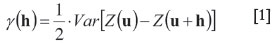
where h is a vector denoting the direction and the Euclidean distance between a pair of locations (e.g. Journel and Kyriakidis, 2004). Although several approaches have been proposed to estimate the semivariogram from the available data, the most commonly used is the unbiased estimator:

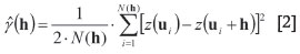
where N(h) is the number of pairs of data values separated by the directional distance h (e.g. Chilès and Delfiner, 2012). This estimator is valid only if the increments (differences) of the regionalized variable are second-order stationary. When the sampling is regular, the calculations are done for multiples of the sampling interval. Otherwise, the distances are grouped into appropriate classes and the effective values of h are the centroids of these classes. The discrete set of (h) values is called variously the sample, experimental, or empirical semivariogram. Semivariogram is also sometimes shortened to 'variogram' in the literature.

For any distance, the ultimate aim is to infer the underlying (or population) semivar-iogram from a sample. The traditional solution is to fit an analytical model to a set of (h)values. The type of model is restricted to those that ensure positive definiteness of variance-covariance matrices in subsequent calculations, which ensures that the solution exists and is unique when the matrix is used in kriging equations. Commonly used semivariogram models include the spherical, exponential, and Gaussian (e.g. Olea, 2009). To maximize consistency between models and data, model parameters are obtained by fitting the model equations to the experimental points either (a) semi-manually with the assistance of graphical software in which the goodness of fit is decided visually, or (b) automatically by using some sort of optimization method. It is often the case that: (i) there are too few pairs for a given distance, (ii) the empirical semivariogram is noisy, and (iii) the data are not normally distributed.

The objective here is to describe the results of work conducted to overcome some of the problems with the two-step approach of calculating semivariogram values and fitting a model, in particular, to: (a) minimize discrepancies between the underlying and the modelled semivariograms, (b) propose a method that is resistant to data preparation errors and robust to departures from normality, and (c) quantify the uncertainty of the estimated model parameters. The results are improvements over previous efforts (Pardo-Iguzquiza and Olea, 2012) in the sense that:

►The bootstrap semivariogram is proposed for inferring the semivariogram model (i.e. semivariogram parameters)

►A procedure is proposed for building confidence intervals

►The bias, variance, and mean square error for the semivariogram parameters are given for a synthetic random field for which semivariogram parameters are known

►The robustness and resistance of the proposed approach are analysed.

 

Robustness and resistance

Equation [2] is a quadratic estimator. Consequently, although theoretically unbiased, it shares all the problems of such estimators, including sensitivity to (a) small sample sizes, (b) skewness in the sample distribution, and (c) presence of outliers. We apply three techniques to mitigate the effect of these factors.

Bootstrap

For a given sample size, n, the bootstrap allows the generation of new samples of the same size. This is accomplished by resampling the sample data-set with replacement, producing multiple data-sets of size n. The new data-sets tend to be all different because in any given resampling some values will be sampled more than once and some will not be sampled at all (e.g. Efron and Tibshirani, 1994). These new samples - called bootstrap samples or resamples - are intended to mimic the results that would have been obtained from other samples that could have been drawn from the random field.

Given a sample of size n, the bootstrap is a method for predicting the dispersion in results that would occur if all possible samples of the same size n were drawn from the population. The classical bootstrap steps for identically distributed and independent values are:

1. Select at random and with replacement n values from the available sample

2. Use the resample values to calculate any statistic of interest, say, the mean, and store the results

3. Go back to Step 1 and repeat the process a large number of times, at least 1000 times

4. Stop.

The set of values generated in Step 2 is the numerical approximation of the variability in the parameter that would be obtained by actually collecting multiple samples of size n.

If the data are spatially correlated then the bootstrap resamples will not be independent and the assumption will be violated. Therefore the application of the bootstrap to spatially correlated data requires two additional steps. First, the spatial correlation must be removed to satisfy the requirement that the values are independent. Once the resample is obtained, the spatial correlation must be re-introduced (Solow, 1985; Pardo-Igúzquiza and Olea, 2012). The effectiveness of the first step could be tested by the p-values of a decorrelation test of normal scores as described in Pardo-Igúzquiza and Olea (2012). However, this has not been pursued further in the proposed approach.

For samples that include abnormally high values, the bootstrap can produce other more typical resamples. By doing so, the values of the parameter of interest, the semivariogram in our case, will also be less extreme and closer to the underlying value, which is the ultimate objective of any statistical inference. The bootstrap filters extreme values by exclusion.

Normal score transformation

The normal score transformation is a bijection between the sample distribution and a standard normal (Gaussian) distribution (e.g. Olea, 2009). Given a sample of size n, it is always possible to rank the values to obtain n quantiles. The bijection is the operation by which the ithmeasurement in the sample is assigned the value of the standard normal distribution for the same ith quantile. Thus, for example, if 20.8 ranks 50 in a sample of size 200, its normal score transformation is -0.675. Most formulations in statistics are either strictly valid for normal distributions or behave better when the sample is normal. The normal score transformation, for example, minimizes the influence of values in the high tail of a positively skewed distribution by scaling the entire sample distribution. The transform reduces the impact of outliers by rescaling to a normal distribution.

The median

The median is the value that divides a sample into two classes of low and high values, each with the same number of measurements. Thus, the median is completely insensitive to changes in observation ranking that do not result in a move from one class to the other. For example, if the median is 45.5 and an observation of 60.9 is erroneously coded as 609, the error has absolutely no effect on the median. If instead, it is miscoded as 6.09, the median does change, but only slightly, to the nearest value below 45.5, say, 44.8. The resistance of the median to these types of changes or to true abnormally high values contrasts significantly with the sensitivity of quadratic statistics (e.g. Cox and Pardo-Igúzquiza, 2001), such as the variance or the semivariogram, particularly to changes in the upper tail of a distribution. Thus, the median buffers the results from outliers.

In a loss function context, the median is the moment that minimizes the sum of absolute errors. In contrast, the mean minimizes the sum of quadratic errors (Klugman et al., 2012).

More than thirty years ago, Armstrong and Delfiner (1980) explored the possibility of estimating the semivariogram in terms of quantiles, but their work has largely been ignored. Other approaches to robust and resistant calculation of semivariograms can be found, inter alia, in Cressie and Hawkins (1980), Cressie (1984), and Dowd (1984).

Performing a fitting to the median of squared differences instead of directly to the empirical semivariogram reduces the sensitivity of the semivariogram modelling to erratic fluctuations. We still use Equation [2] to generate values of an empirical semivariogram as there is no point in using the median for this purpose. The difference here is that the modelling does not stop there. We use the generalized bootstrap to generate multiple empirical semivariograms. The median is used as a measure of central tendency for the set of all bootstrap empirical semivariograms for which the fitting is done.

 

Algorithm

Conformance of the empirical semivariogram with the underlying semivariogram is a necessary condition for the semivariogram model to follow the underlying semivariogram. The general idea is to post-process (filter) the traditional estimator resulting from the application of Equation [2] to remove all the noise that ordinarily causes the empirical semivariogram to deviate from the underlying semivariogram. In this regard, our proposal differs from that of Armstrong and Delfiner (1980) in which the estimator is replaced by the median and the results are corrected to obtain the mean experimental semivariogram.

The algorithm is iterative in the sense of the Kirkpatrick et al. (1983) solution to the classical travelling salesman problem and the simulated annealing of Deutsch and Journel (1998). It comprises two loops, an inner one to generate multiple resamples and an outer one to obtain median semivariograms, as many as necessary to reach convergence. The method stops either when a maximum number of iterations has been reached or the discrepancy between the semivariogram models in the last two iterations is below a threshold. Our approach determines a distance increment to model empirical semivariograms and makes use of two types of analytical models, one for the attribute (B) and another one for its normal scores (A). The iterative steps are:

1. Read in the data

2. Set the number of resamples, the distance interval, the stopping value, and the maximum number of iterations

3. Select the analytical type of the semivariogram model both for the attribute and the normal scores

4. Transform the attribute measurements to normal scores

5. Use a sample of size n to calculate the empirical semivariogram

6. Automatically fit a semivariogram model of type A, which becomes the starting model

7. Use the normal score semivariogram model to calculate the covariance model for all pairs of data locations

8. Apply the Cholesky decomposition to spatially decorrelate the original normal scores to generate a new set of independent normal score values

9. Take a bootstrap resample of the decorrelated values

10. Run a test to check that the normal scores are indeed decorrelated and store the p-value

11. Make the resample spatially correlated by inverting the Cholesky method

12. Calculate the empirical semivariogram for the normal scores and store the results

13. Back-transform the values to their original space

14. Calculate the empirical semivariogram for the resample and store the results

15. Go back to Step 9 if the minimum number of resamples has not been reached. Otherwise, continue to the next step

16. For every distance, take the median value of the estimated semivariogram for the normal scores and for the attribute and then fit corresponding semivariograms of type A and B. If this is the first pass, go back to Step 7. Otherwise, continue

17. If G_iand G_i+1are the last two semivariogram models of type B, calculate

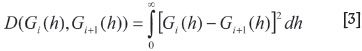
and compare it to the stopping value. If the maximum number of iterations has not been reached and the integral is larger than the stopping value, go back to Step 7. Otherwise, stop; G_i+1 is the semivariogram model for the attribute.

In general, the analytical expression for the semivariogram of the attribute and that of its normal scores may be different and certainly unknown (Stefanou et al., 2004). The algorithm can be simplified for the case when the semivariogram of interest is for the normal scores or for normally distributed values.

The normal scores in Steps 8 and 9 are perfectly decorrelated if, and only if, the semivariogram used to define the correlation matrix is exactly the underlying semivariogram (Hoeksema and Kitanidis, 1985). If the user is interested in investigating the mathematical goodness of alternative semivariogram models, the p-value offers an adequate criterion for comparisons.

 

Case study

Exhaustive sample

A simulated realization of a Gaussian random field is used as an exhaustive sample at a finite number of experimental locations. The advantage of using a synthetic example is that the underlying semivariogram parameters are known and thus the performance of the estimators can be compared in terms of bias, variance, and mean square error. Furthermore, the simulated realization is guaranteed to follow the imposed model, whereas a natural phenomenon will do so only in an approximate manner. Figure 1 shows a realization of a second-order stationary, zero-mean, Gaussian random field with an exponential semivariogram with range 10 units, nugget variance 0.3, partial sill of 0.7, and thus total variance of 1.0. The realization in Figure 1 comprises a grid of 128 x 128 locations with unit grid sides in the X and Y directions. All 16 384 values on the grid were used to calculate the exhaustive experimental semivariogram for the realization shown in Figure 2, together with the model fitted to it:

 

 

 

 

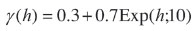
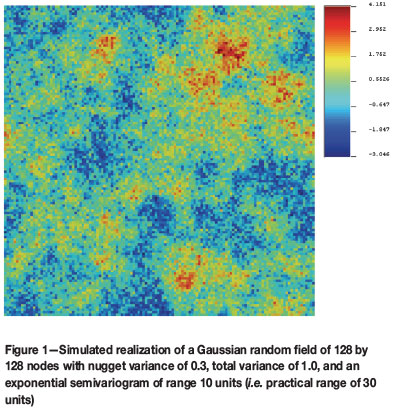
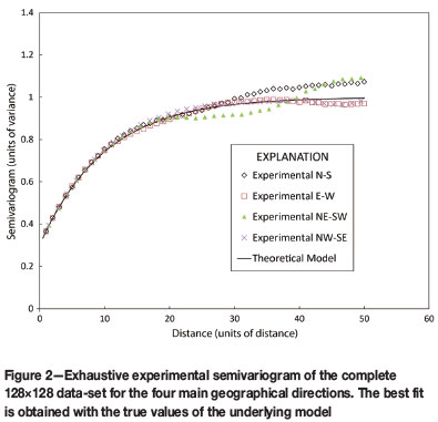
which is the exact theoretical model used to generate the simulation.

In practice, of course, an exhaustive sampling is not possible and, in most geoscience applications, the total sample volume is significantly less than 1% of the total volume from which the measurements are taken. For example, a quartz-vein hosted gold deposit extending over an area of 900 m x 300 m and a vertical extent of 150 m would typically be sampled for reserve estimates on a drilling grid of 30 m (along strike) x 15 m (across strike). Assuming that each drill-hole is 150 m in length and that the diameter of the core is 10 cm, the total sample volume represents 0.002% of the total orebody volume. The proportion of samples does, of course, have to be tempered by the range of spatial correlation and the nugget effect to account just for the independent amount of information in the sample, thus reducing even further the sample representativity. In the synthetic simulated example reported here for demonstration purposes, we have considered primarily samples of size 50, which are: (a) 0.3% of the total possible number of samples that could be taken, and (b) on average, 18 units away from the nearest neighbour, or 60% of the effective range of 30 units. The analysis included samples up to size 200 in some cases.

Assessment of the new estimator

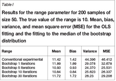
In order to assess the algorithm, a larger number of samples, M, is generated by random sampling from the exhaustive grid of values in Figure 1. For this work we chose 200 (M = 200) for the total number of samples, and 50 (n = 50) for the size of each sample. We specify the semivariogram model as exponential, and compare a conventional model-fitting method to the bootstrapped fitting method. The traditional procedure is to find the exponential model parameters by fitting the model to the experimental semivariogram. Our method calculates the bootstrapped median semivariogram parameters for the exponential model. We then compare the two methods using measures of bias, variance, and mean square error.

For the ith sample, a given semivariogram model parameter θis estimated and the estimated value is denoted . The mean and variance of the estimated parameter values are given by:

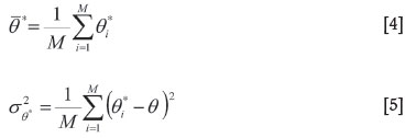
The bias (B) and mean square error (MSE) are estimated as:

and

respectively.

Bias, variance, and mean square error are used to assess the performance of the median semivariogram estimator with respect to conventional estimator (ordinary least-squares fitting of the exponential semivariogram model to the experimental variogram) for several situations of interest. We focus on the most usual semivariogram parameters in the so-called basic Matheron representation: range, nugget variance, and total variance.

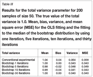
The results of 1, 5, 10, and 30 iterations for a base case are shown in Tables I-III for the three parameters nugget variance, total variance, and range. The decrease in mean square error is different for the different parameters and it is concluded that most of the gain is obtained from the first iteration.

 

 

 

 

 

 

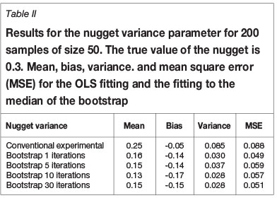
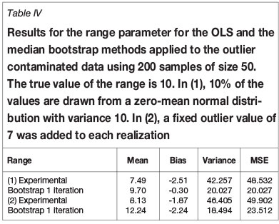
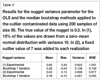
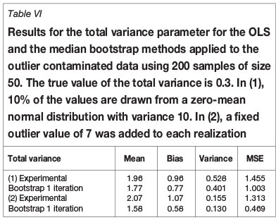
Resistance to outliers was checked by comparing the results using samples from Figure 1 with the results from a contaminated sample. Two contaminations have been used: (a) 10% contamination from a Gaussian distribution with zero mean and variance 10, and (b) adding a single outlier of fixed value 7, which is seven times the standard deviation from the mean. The results are shown in Tables IV to VI for the three parameters of an exponential semivariogram. For the first contamination the bootstrap estimator produces a reduction in the mean square error with respect to ordinary least squares (OLS) for all three parameters. For the second contamination the reduction is smaller, although the contamination model is somewhat naïve.

 

 

 

 

 

 

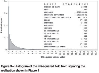
Robustness with respect to departure from the Gaussian distribution was tested by comparing the results obtained when sampling from the Gaussian random field in Figure 1 with those obtained when sampling from the highly skewed chi-squared field resulting from squaring the Gaussian random field. The distribution is skewed as shown in Figure 3, and the range of the exponential covariance is halved so that the new target range is five units of distance.

 

 

The results are shown in Tables VII to IX, from which it can be seen that the median semivariogram estimator has a mean square error that is smaller than that the OLS estimates, but the improvement is not as great as in the Gaussian case.

 

 

 

 

 

 

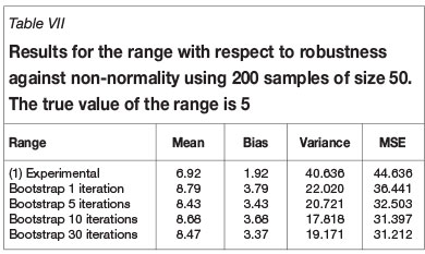
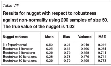
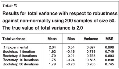
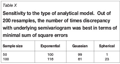
Table X shows the results of a sensitivity analysis of the type of analytical model. All results were obtained assuming the correct exponential model. The method showed some discrimination power for automatically predicting the model type.

 

 

Discussion

Number of samples

For small sample sizes, the new method is an improvement relative to fitting values to (h)from Equation [2], but the improvement declines as the number of samples increases. For 100 data values (or 0.6% of the total possible samples in our case study) the improvement is less than 3% and the results are not significantly different. Nevertheless, there are many important applications that are confined to small data-sets (tens of values) and for which the median bootstrap estimator offers significant improvements. In addition, as noted earlier, in most geoscience applications a sample of 0.6% of the total mass to be sampled is, in fact, a relatively large sample. For the gold orebody example cited earlier, a sample proportion of 0.6% would require a drilling grid of 5 m χ 2.5 m or 36 times more drill-holes, which would be economically unfeasible.

Comparing different semivariogram parameters for the same model

Equation [3] allows the comparison of semivariogram models by redefining G_iand G_i+1as the underlying model and an estimated model. For the case of the exponential model, Table XI shows the results for the same 200 samples used to prepare Tables I-III.

 

 

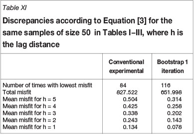
The median bootstrap estimate performs better than the conventional estimate for sample sizes of less than 100. For the 200 samples, the bootstrap models give smaller discrepancies in 116 cases; the total discrepancy is 652.0 against 827.5 for the conventional model fitting and the mean misfit at a distance of half the range (i.e. five units of distance) decreases from 0.50 to 0.31. Thus, using the previous criterion, the model fitted by the bootstrap method is significantly better than the model fitted directly to the values obtained from Equation [2].

Robustness

Robustness with respect to departure from normality is perhaps the best property of the new estimator because, when working with true experimental geoscience data, although the underlying probability density function is almost always unknown, the presence of skewed histograms is the norm rather than the exception.

Resistance

The median bootstrap estimator is resistant with respect to contamination (Tables IV-VI). This is a significant practical advantage as abnormally high values are common in geoscience data and particularly in grade values for mineral deposits. Outliers can significantly and adversely affect the method of moments semivariogram estimator and, for this reason, there is reluctance to using it for analyses and estimations (Krige and Magri, 1982).

 

Uncertainty evaluation

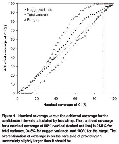
A fundamental objective of any inference method should be to provide the uncertainty of the estimated parameters, especially for small data-sets for which the uncertainty may be large and, consequently, the use of estimated parameters may be meaningless. The most practical way of specifying the uncertainty in an inference problem is by providing probabilistic interval estimates for the parameters. That is, instead of single values, provide an interval containing the true underlying and unknown parameters with a given level of probability. This can be easily obtained from the proposed procedure by fitting a model to each of the 1000 bootstrap samples and then obtaining percentile bootstrap intervals from the bootstrap distribution of the estimated parameters. The median of this bootstrap distribution produces results similar to, but slightly worse than, results from fitting a model to the median semivariogram, and thus this procedure is used only for estimating the uncertainty in the form of percentile confidence intervals. Figure 4 shows the results of an experiment in which the achieved coverage of these confidence intervals was calculated and compared with their nominal coverage. The results show that for low nominal coverage (less than 40%), the achieved coverage is close to the nominal values for the nugget and the range. For high values of the nominal coverage (greater than 65%), the achieved coverage is close the nominal coverage for the total variance parameter and the coverage is overestimated (i.e. on the safe side) for the nugget variance and range parameters.

 

 

Sensitivity to type of analytical model

All results were obtained by assuming the correct exponential model. In a real case study, however, in general the type of model is unknown. Particularly for small data-sets, the significant scatter of the experimental values provides scope for assuming different analytical models. In addition to estimating the underlying parameters, we tested the capability of the methodology to predict the correct functional form of the semivariogram. The testing was limited to three basic choices: exponential, spherical, and Gaussian. Table X shows the number of times each model produced the best result, defined as the best fit to the set of points defining the resulting median semivariogram. In this case at least, the method showed limited discrimination power, indicating that it was insufficient to rely on an automatic prediction of the model type. This ability, however, improved with the sample size.

 

Conclusions

A new approach to modelling the semivariogram estimator has been proposed: the median bootstrap semivariogram. The new method is an improvement on the conventional approach of directly fitting a model to a few empirical semivariogram values. According to an evaluation based on a synthetic exhaustive sample, the improvement is significant mainly for small sample sizes (with n less than 100, or 0.6% of the total possible samples, for the demonstration example). The new estimator has proved to be resistant to slight contamination of the sample distribution and significantly robust to departures from normality. Although further research is required on mathematical proofs, the results are encouraging for incorporating the estimator in computer implementations in which a large number of automatic fittings are required as, for example, when applying moving window statistics in remote sensing, contouring, and other global applications of geostatistics.

 

Acknowledgements

The authors are grateful to Geoffrey Phelps (US Geological Survey) and to Frederik Agterberg (Geological Survey of Canada) for constructive discussion of an earlier version of the manuscript. The work of the second author was supported by the research project KARSTINV CGL2010-15498 from the Ministerio de Economía y Competitividad of Spain. The work of the third author was supported by Australian Research Council Discovery Project grant DP110104766.

 

References

Armstrong, M. and Delfiner, P. 1980. Toward a more robust variogram. A case study on coal. Technical Report N-671, Centre de Géostatistique, Fontainebleau, France.         [ Links ]

Chilès, J.-P. and Delfiner, P. 2012. Geostatistics-Modeling Spatial Uncertainty. 2nd edn. John Wiley & Sons, Hoboken, NJ. 699 pp.         [ Links ]

Cox, M. and Pardo-Igúzquiza, E. 2001. The total median and its uncertainty. Advanced Mathematical and Computational Tools in Metrology V. Ciarlini, O., Cox, M.G., Filipe, E., Pavese, F., and Ritchter, D. (eds.). World Scientific Publishing Company, Singapore. pp. 106-117.         [ Links ]

Cressie, N. and Hawkins, D. 1980. Robust estimation of the variogram: I. Mathematical Geology, vol. 12, no. 2. pp. 115-125.         [ Links ]

Cressie, N. 1984. Towards resistant geostatistics. Geostatisticsfor Natural Resources Characterisation. Veryl, G., David, M., Journel, A.G., and Marechal, A. (eds.). D. Reidel Publishing Company. Series C: Mathematical and Physical Sciences, vol. 122, Part 1, pp. 21-44.         [ Links ]

Deutsch, C.V. and Journel, A.G. 1998, GSLIB-Geostatistical Software Library and User's Guide. 2nd edn. Oxford University Press, New York. 369 pp. and 1 CD.         [ Links ]

Dowd, P.A. 1984. The variogram and kriging: robust and resistant estimators. Geostatisticsfor Natural Resources Characterisation. Verly, G., David, M., Journel, A.G., and Marechal, A. (eds.). D. Reidel Publishing Company. Series C: Mathematical and Physical Sciences, vol. 122, Part 1. pp. 91-106.         [ Links ]

Efron, B. and Tibshirani, R.J. 1994. An Introduction to the Bootstrap. Chapman & Hall, New York. 456 pp.         [ Links ]

Hoeksema, R.J. and Kitanidis, P.K. 1985. Analysis of the spatial structure of properties of selected aquifers. Water Resources Research, vol. 21, no. 4. pp. 563-572.         [ Links ]

Journel, A.G. and Kyriakidis, P.C. 2004. Evaluations of mineral reserves-a simulation approach. Oxford University Press, New York. 216 pp.         [ Links ]

Kirkpatrick, S., Gellat, C.D., J.R., and Vecchi, M.P. 1983. Optimization by simulated annealing. Science, vol. 220, no. 4598. pp. 671-680.         [ Links ]

Klugman, S.A., Panger, H.H., and Willmot, G.E. 2012. Loss Models: from Data to Decisions. 4th edn. John Wiley & Sons, Hoboken, NJ, 513 pp.         [ Links ]

Krige, D.G and Magri, E.J. 1982. Studies of the effects of outliers and data transformation on variogram estimates for a base metal and a gold orebody. Mathematical Geology, vol. 14, no. 6. pp. 557-564.         [ Links ]

Olea, R.A. 2009. A Practical Primer on Geostatistics. US Geological Survey, Open File Report 2009-1103. 346 pp. http://pubs.usgs.gov/of/2009/1103/        [ Links ]

Pardo-Igúzquiza, E. and Olea, R.A. 2012. VARBOOT: a spatial bootstrap program for semi-variogram uncertainty assessment. Computers and Geosciences, vol. 41. pp. 188-198.         [ Links ]

Solow, A.R. 1985. Bootstrapping correlated data. Mathematical Geology, vol. 17, no. 7. pp. 769-775.         [ Links ]

Stefanou, G., Lagaros, N.D., and Papadrakakis, M. 2004. An efficient method for the simulation of highly skewed non-Gaussian stochastic fields. III European Congress on Computational Methods in Applied Sciences and Engineering. Neittaanmäki, P., Rossi, T., Majava, K. and Pironneau, O. (eds.). Springer, The Netherlands. 15 p., http://www.imamod.ru/~serge/arc/conf/ECCOMAS_2004/ECCOMAS_V1/proceedings/pdf/281.pdf        [ Links ]