DANIE KRIGE COMMEMORATIVE EDITION - VOLUME III

 

Improving processing by adaption to conditional geostatistical simulation of block compositions

 

 

R. Tolosana-Delgado^I; U. Mueller^II; K.G. van den Boogaart^{I, III}; C. Ward^IV; J. Gutzmer^{I, III}

^IHelmholtz Zentrum Dresden-Rossendorf, Helmholtz Institute Freiberg for Resource Technology, Germany
^IIEdith Cowan University, Perth, Australia
^IIITechnical University Bergakademie Freiberg, Germany
^IVCliffs NR, Perth, Australia

 

 

---

SYNOPSIS

Exploitation of an ore deposit can be optimized by adapting the beneficiation processes to the properties of individual ore blocks. This can involve switching in and out certain treatment steps, or setting their controlling parameters. Optimizing this set of decisions requires the full conditional distribution of all relevant physical parameters and chemical attributes of the feed, including concentration of value elements and abundance of penalty elements. As a first step towards adaptive processing, the mapping of adaptive decisions is explored based on the composition, in value and penalty elements, of the selective mining units.
Conditional distributions at block support are derived from cokriging and geostatistical simulation of log-ratios. A one-to-one log-ratio transformation is applied to the data, followed by modelling via classical multivariate geostatistical tools, and subsequent back-transforming of predictions and simulations. Back-transformed point-support simulations can then be averaged to obtain block averages that are fed into the process chain model.
The approach is illustrated with a 'toy' example where a four-component system (a value element, two penalty elements, and some liberable material) is beneficiated through a chain of technical processes. The results show that a gain function based on full distributions outperforms the more traditional approach of using unbiased estimates.

Keywords: adaptive processing, change of suppport, compositions, geometallurgy, stochastic optimization.

---

 

 

Introduction

One of the key usages of geostatistics has long been the prediction of the spatial structure of orebodies. This is used for the evaluation of resources and/or reserves and for further planning of the mining and beneficiation process schedule. For most applications, and until quite recently, metal grade has been regarded as the central property of study and the main objective has been to distinguish between ore and waste. However, recently other properties have come into focus through better analytical methods, such as automated mineralogy (see e.g. Fandrich et al. 2007), and new geostatistical methods considering more complex information, such as kriging of compositions (Pawlowsky-Glahn and Olea, 2004). Two ores with the same chemical composition can have totally different mineralogies and microfabrics, which will result in different recoveries, energy requirements, or reagent consumptions, thus yielding very different mass streams. An ore is thus no longer understood as represented by a single value element, but through a complex microfabric (Hagni, 2008). This perspective allows quantitative insight into relevant properties of different ore and gangue minerals (Sutherland and Gottlieb, 1991), potentially containing poison elements or phases (e.g. Houot, 1983) that modify the efficiency of downstream processing steps or require additional treatment.

Accordingly, processing choices have become more complex. Grade-based studies allow a mere 'beneficiate-or-dump' decision. With the advent of these analytical and methodological advances, it is possible to better adapt processing to the ore mined due to a more profound understanding of the processing required. For instance, good knowledge of microfabric properties can reduce energy consumption, if overgrinding is avoided, which also results in improved recovery by avoiding losses due to poor liberation (Wills and Napier-Munn, 2006). Similarly, accurate information on mineral composition may permit the specification of a cut-off in any separation technique (magnetic, electrostatic, or density-based), optimally weighting recovery and further processing costs. Or depending on the proportion of fines generated during milling, desliming might or might not be necessary. Finally, different concentrations of chemicals might be needed for an optimal flotation process as a function of the composition of the concentrate. These are simple examples of the possible adaptive choices that could be implemented in several steps of the process chain, if the necessary ore feed properties were known. Actually, the complexity of the interactions between the several processes is such that the best processing stream might not be an intuitive one, requiring the solution of large combinatorial problems. Such considerations will become a requirement in the near future, due to the lower margins imposed by a globalized economy.

In most current mining operations, ore is blended to a homogeneous quality based on geostatistical prediction, to ensure optimal performance of a beneficiation route that has been empirically optimized, but that remains mostly constant throughout the mine life. Geometallurgy (Jackson et al., 2011) aims to produce higher overall gains by adapting the processing to the predicted ore quality of the block currently being processed.

The aim of this paper is to demonstrate the use of geostatistics in such a complex processing situation, with particular regard to the following key issues.

►The relevant microfabric information is not captured by a single real number, but typically involves nonlinear and multivariate scales. This is illustrated by analysing compositional data, where a direct application of standard geostatistics can lead to artefacts, including negative concentrations and dependence of predictions on irrelevant components. For example, a non-compositional cokriging of a mineral composition applied to a system that includes both value and waste minerals cannot be transformed in a simple way into an optimal unbiased prediction of the subcomposition of value minerals only (Tolosana-Delgado, 2006), so that waste components separated in the first processing steps have a lasting influence all along the processing chain. These problems are analogous to the wellknown order relation problems of indicator kriging (Deutsch and Journel, 1992; Carle and Fogg, 1996)

►The prediction is used for a nonlinear decision problem, involving geological uncertainty and a processing model. In this context, a decision based on unbiased estimates of the relevant properties is no longer optimal.

To illustrate how geostatistics must be applied in such a situation, an example from a mined-out iron ore orebody is used. Since no systematic adaptive processing has been applied during the exploitation of the mine, a 'toy' example will be used to illustrate possible classes of processing choices and their effect in the geostatistical treatment. A simple processing decision set is presented here, to keep the discussion focused on the methodological geostatistical aspects. Readers should be aware that realistic decision sets will be much more complex.

 

Interpolation of geometallurgical data

Kinds of geometallurgical data

Several kinds of data may be collected to characterize the materials to be mined and beneficiated. Each of these kinds of data has its own scale, that is, a way to compare different values. Typical geometallurgical scales are the following:

►Positive quantities, such as the volume of an individual crystal or particle, or its density, its hardness, or the area or major length of a given section

►Distributions, which describe the relative frequency of any possible value of a certain property in the material. The most common property is size: grain size or particle size distributions, either of the bulk material or of certain phases are the typical cases

►Compositional data, formed by a set of variables that describe the importance or abundance of some parts forming a total. These variables can be identified because their sum is bounded by a constant, or by their dimensionless relative units (proportions, ppm, percentage, etc.). Typical compositions include geochemistry, mineral composition, chemical compositions of certain phases, and elemental deportment in several phases. If the composition of many particles/crystals of a body is available, one can also obtain its compositional distribution. A systematic account of compositions can be found in Aitchison (1986) and van den Boogaart and Tolosana-Delgado (2013).

► Texture data, representing crystallographic orientations and their distributions, for instance the concentration ( i.e. inverse of spread) of the major axis orientation distribution of a schist

►More complex data structures can be generated by mixing the preceding types, for example a mean chemical composition can be characterized for each grain-size fraction, or a preferred orientation can be derived from each mineral type.

All these scales require a specific geostatistical treatment. For instance, classical cokriging of a composition seen as a real vector leads to singular covariance matrices (Pawlowsky-Glahn and Olea, 2004), and even if corrected for this problem, predictions can easily have negative components in minerals with highly variable overall abundances. Putting such predictions into processing models is not sensible. Therefore, ad-hoc geostatistical methods honouring the special properties of each of these scales have been developed. Geostatistics for positive data (Dowd, 1982; Rivoirard, 1990) is well established. Textural data-sets have been studied by van den Boogaart and Schaeben (2002), while one-dimensional distributional data-sets were treated by Delicado et al. (2008) and Menafoglio et al. (2014). Compositional data geostatistics was studied in depth by Pawlowsky-Glahn and Olea (2004) and Tolosana-Delgado (2006), and is applied here.

Some of these kinds of data are not additive, in the sense that the average property of a mining block is not the integral over the property within the block. For instance, the arithmetic mean of mass composition within a block is not the average composition of a block if the density varies within the block, or when some components are not considered, a problem known as subcompositional incoherence (Aitchison, 1986). The lack of additivity is particularly important for spatial predictions of the properties of mining blocks or selective mining units (SMUs). The proposed method will require only that the property - or more precisely its effect through processing - is computable from a simulation of a random function describing the variation of the property within the block.

An additional difficulty to be considered in a general framework of geometallurgical optimization is stereological degradation. Many kinds of data available are measured from 2D sections by automated mineralogy systems (Mineral Liberation Analyser (MLA), QUEMSCAN, EBSD, EMP, etc.), while the relevant target properties are actually their 3D counterparts. Some of these 2D data types are nevertheless unbiased estimates of their 3D properties. Modal mineralogy will belong to this category if it is computed from proportions of grain area of each mineral type with respect to the total area translated into volume ratios of that mineral with respect to the total volume. For many other properties, one should consider the possible 3D to 2D stereological degradation effects, in addition to all other considerations presented in this work.

To avoid introducing the extra complexity derived from stereological reconstruction, this paper focuses on the use of compositional information for geometallurgical characterization, that is, modal mineralogy and chemical composition. Due to the lack of a reference deposit with mineralogical data at a sufficiently fine spatial resolution, the mineralogy was reconstructed from the chemical data. However, in future projects where adaptive processing is planned, it is likely that automated mineralogy will be routinely applied and direct measurements of mineralogy are expected to be the rule, not the exception.

Compositional data

Compositional data consists of vectors x =[x₁, x₂,..., x_D] of positive components that describe the relative importance of D parts forming a total. Compositions are characterized by the fact that their total sum is either an artefact of the sampling procedure, or it can be considered irrelevant. Because of this irrelevance, it is legitimate to apply the closure operation

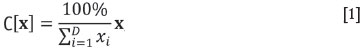
to allow for comparison between compositions.

The most typical compositions in geometallurgy are chemical composition and mineral composition. These compositions can be defined on the same body, and one might require transforming one into the other. If the chemical and mineralogical compositions of a block are assumed to be represented by x^c and x^m, having D^c and D^m components respectively, and each of the minerals is assumed to have a known stoichiometry in the chemical components considered, then the stoichiometry can be realized as a matrix transformation. If the stoichiometry is placed in the columns of a D^c x D^m matrix T, then T maps any mineralogical composition to a chemical composition:

Inverting this equation is called unmixing, and is a part of the broader class of end-member problems (Weltje, 1997). The relation in Equation [2] can be inverted only in the case when D^c = D^c and no chemically possible reactions exist within the system of minerals under consideration (i.e., T is a square matrix and its columns are linearly independent vectors). For D^c > D^m, Equation [2] may not have an exact solution, and one must resort to a least-squares estimate, 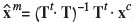, to find the that best approximates x^m. When D^c < D^m,the system will have infinitely many solutions and not all of these will be mineralogically meaningful. Note that these cases do not ensure that the recast composition has positive components. Tolosana-Delgado et al. (2011b) present an algorithm for estimating mineral compositions compatible with observed chemical compositions in all three cases, an algorithm that can also account for varying mineral stoichiometry and ensures that results are positive. For the purpose of this paper, we consider the same number of chemical components as end-members, related through the transfer matrices specified in the section 'Geochemical data and mineral calculations'. Note that in the case D^c = D^m, results can be strongly dependent on the stoichiometry assumed, in which case it could become safer to further treat the geochemical information. On the other hand, the advent of automated mineralogy systems may soon render these calculations unnecessary.

The end-member formalism applies a multivariate analysis framework prone to some fundamental problems of compositions, such as the so-called spurious correlation (Chayes, 1960) induced by the closure operation (Equation [1]). Aitchison (1982, 1986) analysed this difficulty systematically and proposed a strategy for the statistical treatment of compositional data-sets based on log-ratio transformations. The idea is transform the available compositions to log-ratios, for instance through the additive log-ratio transformation (alr):

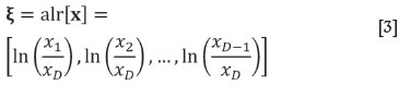
and apply any desired method to the transformed scores Those results that admit an interpretation as a composition (for instance, predicted scores) can be back-transformed with the additive generalized logistic function (agl). The agl is applied to a vector of D - 1 scores, ξ=[ξ₁,ξ₂,..., ξ_D-1],and delivers a D-part composition:

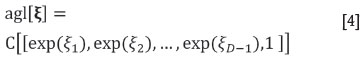
where the closure operation C from Equation [1] is used. This strategy has the advantage of capturing the information about the relative abundance (i.e. abundance of one component with respect to another, their ratio) in a natural way (Aitchison, 1997, van den Boogaart and Tolosana-Delgado, 2013). Another advantage of working on the alr-transformed scores is that, without any need of further constraints, all results represent valid compositions. This was not the case with Weltje's (1997) end-member algorithms, where the final results might present negative components. On the side of the disadvantages, the log-ratio methodology cannot deal directly with components of zero or below the detection limit, and some missing data techniques must be applied, prior to or within the end-member unmixing or (geo) statistical treatment (Tjelmeland and Lund, 2003; Hron et al., 2010; Martín-Fernández et al., 2012). It is often proposed to impute the zeroes by some reasonable values, often a constant fraction of the detection limit. However, for geometallurgical optimization purposes, this imputation by a constant value should be avoided, because it leads to reduced uncertainty scenarios; multiple imputation offers a much better framework accounting for that extra uncertainty (Tjelmeland and Lund, 2003).

Using the log-ratio approach it is possible to define a multivariate normal distribution for compositions (Aitchison, 1986; Mateu-Figueras et al., 2003), with density

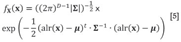
where μand Σare the mean vector and covariance matrix of the alr-transformed random composition X (uppercase indicates the random vector, and lowercase a particular realization). Given a compositional sample {x₁, x₂,...,x_N}, unbiased estimates of these parameters are provided by the classical formulae applied to the log-ratio transformed scores:

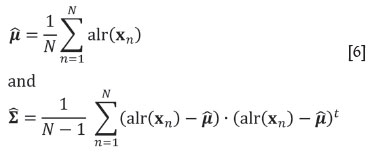
The mean vector estimate can be back-transformed to the compositional centre, cen, which is an intrinsic property of X, not depending on the alr transformation used to calculate it (taking a different denominator would produce the same compositional centre).

Regionalized compositions

Following the principle of working on alr-transformed scores, the classical multivariate geostatistical framework can be applied to compositions (Pawlowsky-Glahn and Olea, 2004; Tolosana-Delgado, 2006; Boezio et al., 2011, 2012; Ward and Mueller, 2012; Rossi and Deutsch, 2014). In this section the relevant notation is introduced and several particularities are clarified that arise from the nature of compositional data. Assume that an isotopic compositional sample is available {x(s₁), x(s₂),..., x(s_N)} at each of a set of locations {s₁, s₂,..., s_N} within a domain E, and for each location s_a denote by ξ(s_α)= alr(x(s_α)) the corresponding alr-transformed composition. Then as with the covariance in Equation [6], experimental matrix-valued alr-variograms can be estimated by conventional routines as semivariances of increments of log-ratio-transformed data.

A linear model of coregionalization Γ(h) (Journel and Huijbregts, 1978; Wackernagel, 2003) is fitted to the experimental alr variogram, expressed as

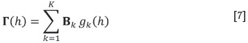
where K denotes the number of structures. For each structure k, 1≤ k ≤ K, the function g_k is an allowable semivariogram model function and the matrix B_k is its associated positive semi-definite covariance matrix. Alternative ways exist for estimating the LMC and ensuring its validity without using any specific alr transformation (Tolosana-Delgado et al., 2011a; Tolosana-Delgado and van den Boogaart, 2013). As usual, a covariance model C can be linked to the variogram through C(h) = C(0)- Γ(h) (Cressie, 1993), assuming second-order stationarity of the log-ratios.

Once a valid LMC for the alr variables is available, kriging estimates can be computed. As in the case of classical multivariate geostatistics, estimates of the alr variables can be made at unsampled locations using the covariance structure defined in Equation [7]. For example, the local neighbourhood simple cokriging estimate ξ^*SK(s₀) at location s₀ is given by

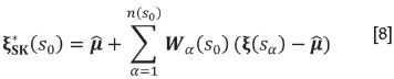
where is the mean of the alr-transformed data, W_α(s₀) is the matrix of weights derived from the simple cokriging system (e.g., Myers, 1982), and n(s₀)is the number of data locations forming the local neighbourhood relevant to predicting x(s₀). The kriging estimates ξ^*(s_α) need to be back-transformed to a composition. A simple approach for doing so is to use the agl transformation, which provides a slightly biased back-transform of the results; an alternative method is to apply Gauss-Hermite quadrature to compute an estimate of the expected value of the composition, assuming that it has a normal distribution (Equation [5]) specified by the cokriging predictor and its cokriging variance. In estimation procedures, that option would be preferable, and the interested reader is referred to Pawlowsky-Glahn and Olea (2004) or Ward and Mueller (2012) for details. However, simulation is more relevant for the goals of this paper, as it allows at the same time an upscaling of the output to block estimates.

In what follows it is assumed that the compositional data does not show gross departures from joint additive logistic normality (Equation [5]). In practice, this happens to be more restrictive than one would think, and a transformation to normal scores is required prior to simulation. The current accepted geostatistical workflow includes applying a normal-score transform to each variable separately (in this case, to each alr-transformed score). Although this guarantees only marginal normality and not joint normality, until recently there were no practical alternative methods that deliver a multivariate jointly normal data-set. Stepwise conditional transformation (Leuangthong and Deutsch, 2003) is not practical for high-dimensional data-sets, and the projection pursuit multivariate transform (Barnett et al., 2014), a recent approach that promises to remedy this shortfall, could not be implemented here as it appeared only during the review process.

For simulation, the turning bands algorithm (Matheron, 1973; Emery, 2008; Lantuéjoul, 2002) is particularly efficient in a multivariate setting as it can be realized as a set of univariate unconditional simulations based on the LMC fitted to the alr or normal-score transformed data and only a single cokriging step is required.

Assuming that the LMC for the data is given by Equation [7], each structure is simulated separately making use of the spectral decomposition of the corresponding coefficient matrix of the LMC. A Gaussian random field can be simulated by putting

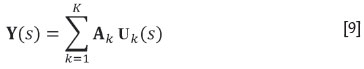
where U_k is a vector random field with D-1 independent components for each k, 1≤ k ≤K. Because of the independence of the components, the simulation of the random field Y reduces to the simulation of K univariate Gaussian random fields, U_k, 1 ≤k ≤K. These are simulated separately using the turning bands algorithm and then re-correlated via Equation [9]. This produces at each location s and at each data location a simulated vector y(s) with the specified spatial correlation structure. Then, simple cokriging (Equation [8]) of the residuals ε(s_n)= y(s_n)- ξ(s_n) at the sample locations s_n, 1≤ n ≤N, is used to condition the realizations through ξ(s₀) = y(s₀) + ε*(s₀) for each location s₀ of the simulation grid. Finally, an agl (and/or a Gaussian anamorphosis) transformation is applied to back-transform the conditioned vectors to compositional space, x(s₀) = agl(ξ(s₀)).

Monte Carlo approximation to compositional block cokriging

A common problem of geostatistics applied to any extensive variable with a non-additive scale is the lack of a universal model of change of support - that is, a way to infer the properties of a large block from much smaller samples. For positive data, for instance, Dowd (1982) and Rivoirard (1990) offer methods for estimating the average grade value within a block, mostly assuming a certain preservation of lognormality between the samples and the blocks. For the other geometallurgical scales, geostatistical simulation offers a general computationally-intensive solution, albeit not an impossible one with modern computers and parallel code. This is illustrated here again for a compositional random function.

Assuming that the random function X(s) can be defined at any differential block du, its average within a block v centred at the position s is

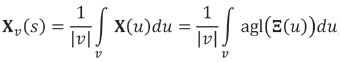
with |v| denoting the block volume, and Ξ(s) = alr(X(s)) the alr-transformed random function. Block cokriging would deliver an estimate of , which is not a good stimate of X_v(s) due to the nonlinearity of the alr-transformation. Instead of block cokriging, the block is discretized into M equal-volume units, and the corresponding pointsupport random function is simulated at their centres. If there are J realizations, then for each j, where 1 ≤ j ≤J, averaging over the units within the block results in an estimate

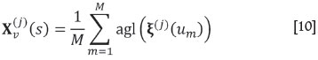
where ξ^(j) (u_m) denotes the alr vector at location u_m∈ v, 1≤ m ≤M drawn in the j-th simulation. This approach has the further advantage of also delivering information about the distribution of x_v(s), not just an estimate of its central value,

Tolosana-Delgado et al. (2014) propose to simulate these alr vectors using the LU decomposition method (Davis, 1987), which is able to produce a large number of replications with minimal cost (large J), but can handle only a limited number of locations (small N + M). This is convenient for obtaining independent estimates of each block, as only simulation within it is needed. Alternatively, if the block estimates are intended to guide global choices, as is the case here, the use of a global simulation like the turning bands algorithm is preferable.

 

Modelling optimization problem

Processing model

Within the framework of Coward et al. (2009) distinguishing between primary variables (intrinsic properties of the natural materials) and response variables (results of human manipulations of the material), the block mean composition X_v(s) can be understood as a primary variable, while the benefit or gain G(X_v(s), C(s)) is the ultimate response variable, a function of the primary properties of the block s and of all choices C(s) taken during its processing. From this point on, the block support taken will be assumed to correspond to the processing unit, i.e. that volume that may be assumed to behave additively as a homogeneous mass through the process chain. Moreover, the true primary properties are usually not available, because they were interpolated/extrapolated from nearby information or because they are not measurable at all (like size distribution information, affected by stereological distortion). In these cases, one has only estimates, nearby observations, or even indirect or proxy measurements of the target primary properties, jointly denoted as Z. Many of the kinds of geometallurgical data discussed earlier are direct proxies for primary variables, with the notable exception of data on particle properties (which already depend on which kind of breakage was applied, and are therefore response variables). The choice C(s) may denote a complete decision tree, with a complex combination of multiple sub-choices. As such, it might encode the processing sequence (like whether or not to include an extra flotation step) and operational parameters (like the cut-off density selected for density separation), but it can also be a simple on/off choice of processing the material or dumping it as waste.

Once the processing options have been determined for a block v centred at location s, the option yielding the largest gain must be found. A typical approach would be to replace the true material property X_v(s) in the gain function by its unbiased estimate based on the available data Z, i.e. the estimate with . This has been shown to be a poor decision rule (van den Boogaart et al., 2011). Given that X_v(s) is uncertain, that naïve approximation would be equivalent to assuming

which is identically true only if either X_v(s) is a known constant, or the gain G(X_v(s), C(s)) is a linear function of X_v(s). Given that the gain function is usually piecewise defined (see the 'Illustration example' section) and that recovery portions are bounded by 0 and 1, one cannot expect linearity to hold.

Maximizing the expected gain

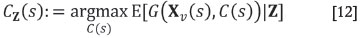
According to van den Boogaart et al. (2013), the best choice C_z(s) for processing the block at location s given the data Z is computed by maximizing the expected gain with respect to the available decisions conditional on the data:

This requires computing the conditional expectation of the gain given the data for each possible choice, readily available from J conditional simulations obtained from Equation [10], through a Monte Carlo approximation:

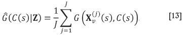
Having computed the gain for each choice, one can then select the choice yielding the largest gain.

Decision-making in mining is rarely based exclusively on the properties of the individual blocks. Rather, many choices are global decisions, i.e. non-adaptive choices that affect the entire domain E. This requires maximizing

which can also be estimated within the same framework by Monte Carlo approximation of the gain

with the domain discretized into B blocks, each centred at a location s_b, 1≤ b ≤ B. This category of global choices includes the setting of quality thresholds, blending strategies, design throughput, or the block extraction sequence. These aspects are not treated in this paper.

 

Illustration example

Geological description

The data-set used comes from a high-grade iron ore deposit (K-pit deposit, see description by Angerer and Hagemann, 2010) hosted by banded iron formations of the Archean Koolyanobbing Greenstone Belt, Western Australia, located 360 km east of Perth in the Southern Cross Province of the Yilgarn Craton. The greenstone belt strikes northwest and is approximately 35 km long and 8 km wide. It is composed of a folded sequence of amphibolites, meta-komatiites, and intercalated metamorphosed banded iron formation (BIF; Griffin, 1981). The K-deposit occurs where the main BIFhorizon, striking 300° and dipping 70° NE, is offset by younger NNE-striking faults (Angerer and Hagemann, 2010). The resource of the K-deposit consists of different mineralogical and textural ore types, including hard high-grade (>55% Fe) magnetite, haematite, and goethite ores and medium-grade fault-controlled haematite-quartz breccia (45-58% Fe) and haematite-magnetite BIF (45-55% Fe).

Three domains, 202 (west main domain), 203 (east main domain), and 300 (haematite hangingwall) were selected as they can be considered reasonably homogeneous from a mineralogical point of view: the iron-rich facies is dominated by haematite in all of them, with minor contributions from magnetite or goethite/limonite.

Geochemical data and mineral calculations

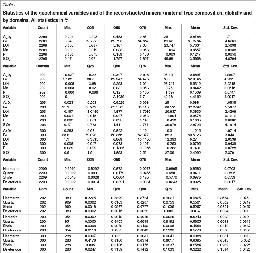
Six parameters were considered for analysis: Fe, LOI, Mn, SiO2, P, and Al2O3, as well as the residual to 100% not accounted for by these. The residual should be considered equal to the mass contribution of the remaining elements not reported here: for example, oxygen from the various Fe and Mn oxides, or OH and Ca from apatite. Thus, the number of original components is D^c=7. Table I summarizes the main characteristics of this data-set.

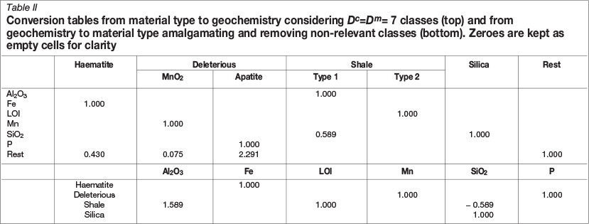
The chemical compositions were converted to mass proportions of the following D^m= 7 mineralogical-petrological reference material types as end-members (amalgamated then in four types):

►Haematite (Hm), taking all the Fe in the chemical composition, and as much of the residual as required for haematite (Fe₂O₃)

►Deleterious (Dl), adding up two contributions:

- Mn oxides, whose mass proportion was computed using all Mn and the necessary oxygen from the residual in a molar proportion of 1:4 (giving a mass proportion of 1:0.0751)

- Apatite, with an ideal composition Ca₅(PO₄)₃(OH), where again the mass proportion of P was increased by removing the necessary mass from the residual (to account for Ca, O, and OH)

►Shales (Sh), again with two contributions:

- The whole LOI mass contribution (because goethite/limonite contribution to Fe is negligible in the chosen domains), and

- All Al₂O₃, together with a 1:1 mass proportion of SiO2 (equivalent to 10:6 in molar proportion, i.e. an Al-rich material type)

►Silica (Qz), equal to the residual SiO₂ not attached to shales

►Residual, equal to the remaining residual not attributed to any of the preceding classes. This can be disregarded, because it is assumed to be inert and it represents an irrelevant small mass input to the system.

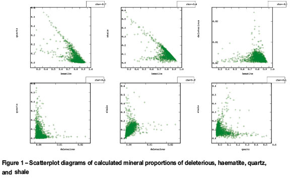
Table II summarizes the transfer matrix from material types to geochemistry. The proportions of the four types can be computed from the (generalized) inverse of the transfer matrix. None of the resulting four main components was negative, and the residual disregarded component always dropped to zero (accepting an error of ±2%). Material type proportions obtained are shown in Figure 1, and Table II summarizes their statistics also.

 

 

Devised toy processing

Although the K-deposit was exploited without any processing beyond crushing and (eventually) screening, in this contribution a reasonable selection of processing choices was assumed for BIF-hosted iron ores (Houot, 1983; Krishnan and Iwasaki, 1984), with the aim of illustrating what can be expected from the proposed geostatistical method of geomet-allurgical adaption.

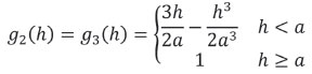
Selective mining units (SMUs) are considered to be volumes of 12x12x6 m³. If an SMU is considered economically interesting, it is processed as follows (Figure 2). First, the SMU is extracted, transported, and crushed by a primary crusher. This represents fixed costs of Q₀. Here it is assumed that all material containing more than 88% haematite will be a lump product, i.e. particle size greater than 6.3 mm and less than 31.5 mm. An SMU with an average haematite content greater than 88% (i.e. more than 60% Fe), is considered to be in this lump category. Otherwise, the product is sent for further grinding (costing an extra Q_f), and will be considered as fines. Usually, the definition of lump depends on other geometallurgical properties (hardness and grain size), but for the sake of simplicity this has not been taken into account here.

 

 

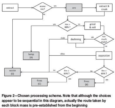
Material that is not considered to be lump can be processed through a desliming process, depending on the proportion of shale. If desliming is switched in, the amount of shale is assumed to be reduced by 15%, with the rest of the components unchanged. Desliming costs are Qdmonetary units per volume washed, independent of the actual amount of shale. Thirdly, the product is fed to a separation process (for instance, flotation), devised to remove quartz: 100% of the quartz, together with 10% of shale and 30% of haematite and deleterious components, is sent to the tailings. Separation costs per unit of material recovered are denoted as Q_s. The product must then be classified into high-grade fines (more than T_h= 85% haematite in the product), low-grade fines (haematite with T_l= 80% or more), or waste. The different products are sold at different prices: I₀ for lump, I_hfor high-grade fines, I_lfor low-grade fines, and zero for waste.

Table III summarizes the quantities used for these monetary values. The prices and the partition coefficients considered for each phase through desliming and separation were chosen to enhance the contrast between the proposed methodology and the classical one. The calculations proposed here can be adapted to current market prices by changing these constants.

 

 

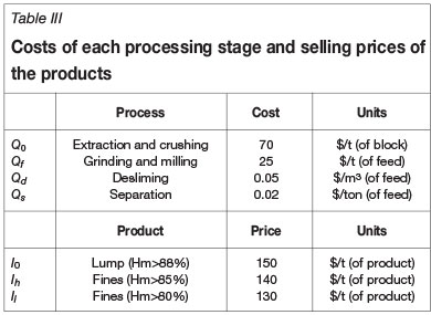
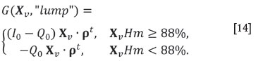
The first choice is to process or dump the block. If processed, the following costs will be incurred. Denoting the original block composition in terms of the four components [Hm, Dl, Sh, Qz]by X_v (the spatial dependence is dropped here for the sake of simplicity), and considering ideal densities of each of these materials respectively as ρ_Hm = ρ_Dl= 3.5 t/m³ and ρ_Sh= ρ_Qz= 2.5 t/m³ within a vector ρ= [ρ_Hm,ρ_Dl, ρ_Sh, ρ_Qz], the cost of crushing and transporting a block of unit volume is Q₀X_v· ρ^t,using the dot product notation for product of matrices. Note that the result is in this case a scalar value. The second choice is to sell the processed block as the category 'lump' or further process it. Selling as lump produces an income of I₀X_v ρ^tif the material fulfils the quality requirements. The gain of selling it as lump is thus

If the product is not sold as lump, it must be further ground, which represents a cost of Q_fX_v· ρ^t.The following choice is to apply a desliming process, which costs Q_d. Its effect is to modify the mass proportions to X_d= X_v* [1, 1, 1, 0.85], where * denotes the direct product (i.e. component-wise product of the two vectors). Note that this is analogous to a filter, i.e. a process where the partial output concentration is obtained by keeping a known different portion of each input component. Then, a separation process is applied, which represents a similar filter to a vector of masses X_s= X_v* [0.7, 0.7, 0, 0.9] with cost Q_sX_v· ρ^t if no desliming was applied, or to X_ds= X_d* [0.7, 0.7, 0, 0.9] costing Q_sX_s· ρ^tif desliming was switched in. Finally, one must choose the quality at which the product is desired to be sold, choosing between high (X_sHm ≥T_h =85%) and low qualities (T_l = 80% ≤X_sHm < T_h= 85%). If no desliming was applied, this produces four options:

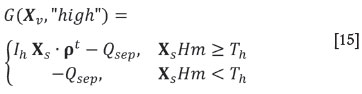
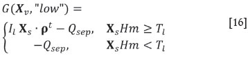
being Q_sep= (Q₀+ Q_f+ Q_s) X_v· ρ^t; or if desliming was necessary

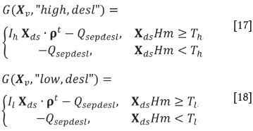
where Q_SepdeSl = (Q₀ + Q_f) X_vρ^t+ Q_d + Q_s X_s·ρ^t.Note that all these costs, incomes, and gains are expressed for blocks of unit volume, so that they should be multiplied by 12 · 12 · 6 m³ if one wishes to refer them to an SMU.

Results

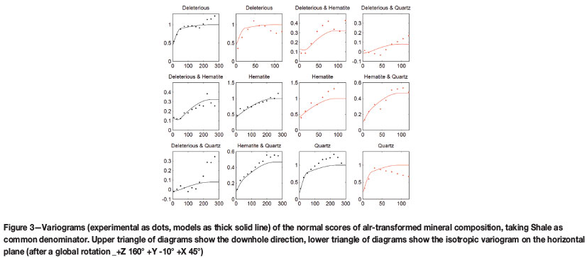
Following the geostatistical procedure for compositions outlined before, the alr transformation was applied (Equation [3]) to the material composition Dl-Hm-Qz-Sh, taking shale as common denominator. To better approach the required normality in simulation algorithms, alr variables were converted to normal scores via a normal scores transform, and the variograms of the resulting scores were estimated (Figure 3) and modelled with an LMC (Equation [7]) consisting of a nugget and two spherical structures, i.e. using a unit variogram

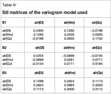
with the first range α= 52 m in the plane (and an anisotropy ratio vertical/horizontal of 23/52) and the second range α= 248 m in the plane (and an anisotropy ratio vertical/horizontal of 94/248). Table IV reports the sill matrices B₁(linked to the nugget), B₂, and B₃ of this model. Note that a global rotation along +Z 160° -Y 10° +X 45° (mathematical convention) was applied.

 

 

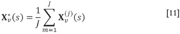
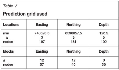
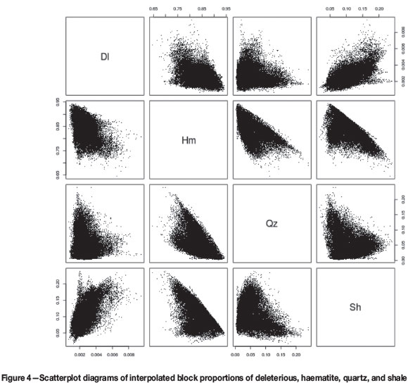
An SMU grid was constructed such that no block was more than 50 m away from a sample location. Each of the resulting 33 118 blocks was discretized into 4 x 4 x 2 = 32 points, oriented along the natural easting-northing-depth directions. The SMU grid and the underlying point grid are described in Table V. Using a turning bands algorithm, 100 non-conditional simulations were obtained and conditioned via simple cokriging. The conditioning step was succeeded by the application of the Gaussian anamorphosis and the agl transformation (Equation [4]) to obtain values for the four-material composition, which were then averaged in accordance with Equation [10]. This provided 100 realizations of the average composition for each block. Figure 4 shows the scatter plots of mean values of block averages of these simulations after applying Equation [11]. A comparison with the spread of the original data (Figure 1) shows a satisfactory agreement of both sets, and that the obtained block average estimates show similar constraints as the original data.

 

 

 

 

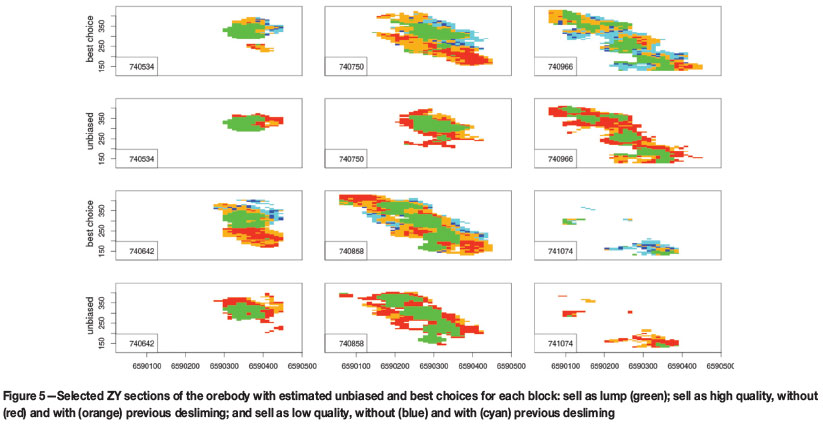
Two methods for decision-making are compared in what follows. First, for each block Equations [14]-[18] were applied using the block averages computed previously. Then, each block was treated with the choice that produces the largest gain out of the five options available. Figure 5(right) shows a selection of ZY sections of the domain, where the colour of each block depends on the treatment chosen according to this average unbiased estimate. This represents the approach of choosing the treatment on the basis of the best available unbiased estimate of the primary properties.

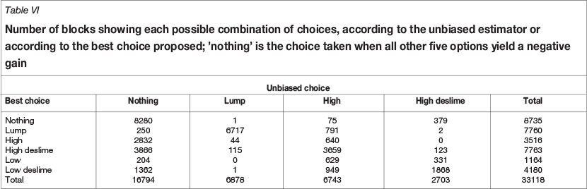
Secondly, the gain was calculated for each simulation and then averaged via Equation [13]. For each block, the option yielding the largest average gain was chosen. This represents the proposed approach of maximizing the conditionally expected gain. Figure 5 (left) shows also the same sections of the domain, using the same set of colours but now defined according to the proposed criterion. Table VI summarizes the two choices for each block (after the unbiased estimate and after the proposed criterion). From Figure 5 and Table VI, it is immediately obvious that the proposed criterion promotes a much more thorough exploitation of the deposit, prescribing more treatment and suggesting selling part of it at lower prices.

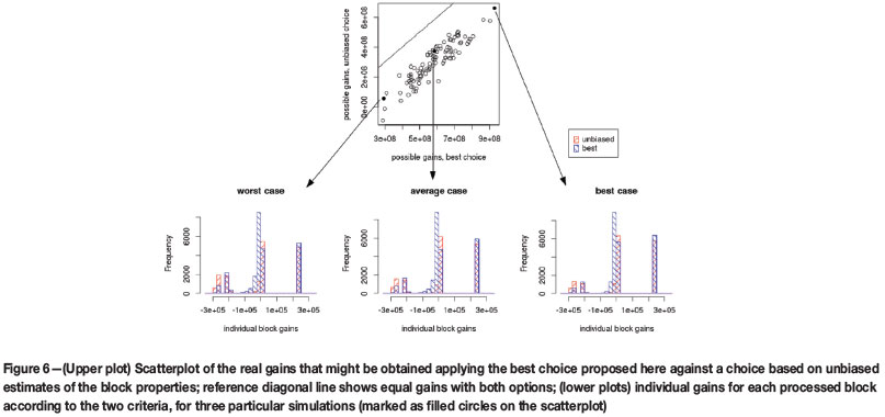
Finally, for each of the 100 simulations, the gains for the entire domain were computed using both approaches. These are compared in Figure 6, where it is clear that the proposed criterion always delivers a larger gain than the unbiased estimator criterion. Figure 6 also shows histograms of the gain (and loss) contribution of each individual block for three selected ranked simulations (representing a poor deposit, an average deposit, and a rich deposit, all three scenarios compatible with the available data). These histograms show that the individual gains are very different, typically: a large gain (around 2.5 · 10⁵), a minimal gain (>0), a minimal loss (<0), and moderate-large losses (two subgroups, around -2 · 10⁵and -3 · 10⁵). The histograms show that, with respect to the unbiased estimator choice, the best choice primarily reduces the large losses (increasing slightly the minimal losses) and slightly increases the large gains.

 

Discussion

The results suggest that mean block unbiased estimates deliver poor choices because of the asymmetry of the gain function. A synthetic example might explain why this happens. If one considers all blocks for which the estimated haematite average content is slightly above the lump threshold (Hm>88%), then the unbiased choice would immediately consider all of them as lump, but each could be sold only if its real haematite content was greater than 88 wt%. This means that, depending on the uncertainty on the real haematite content, some of the blocks will actually fall below the threshold, and cannot be sold at the expected price (thus incurring non-realized gains). In contrast, if all blocks are considered whose estimated haematite content is slightly below the threshold, then all of them will be sold at the 'high-quality' price, and those whose real haematite content would qualify them as 'lump' will be sold at this lower price. In other words, the effects of these two errors ('high quality' taken as 'lump', and 'lump' taken as 'high quality') do not compensate one another, and the result is a net loss with respect to that predicted by plugging the unbiased estimate into the gain function. With more thresholds and more decisions this effect accumulates, producing systematic losses in each classification step.

The proposed criterion essentially minimizes the loss, often by reducing the threshold at which the product is considered economic. In that way, though more 'high quality' is classified as 'lump' and extracted but not sold (thus resulting in some loss), also more 'lump' is properly classified and sold at the higher price, (more than just compensating the potential losses). The same can be seen in the prediction of low-quality blocks: the optimal criterion proposes to process many blocks for which the estimated average haematite content is slightly below the threshold of minimal quality (Hm>80%), because those of them that are above the threshold will pay for the extra costs of processing those that are actually below the defined threshold. In real applications, this concept would be used for the whole deposit, in order to look for those quality thresholds (fixed to 88%, 85%, and 80% here) that after blending each quality class would maximize the global gain. This global optimization was left for further research, to keep the discussion simpler, but readers should be aware that optimizing blending is one of the most important choices in terms of global impact on the gain.

The modification of the threshold can also operate in the other direction, as it depends on the uncertainty attached to each estimate, and the differences between gains and losses for each misclassification. This can be inferred from two aspects seen in Figure 5. First, desliming a block that according to its average value would not require desliming is considered by the unbiased criterion as a waste of money, thus almost no block is deslimed here; on the other hand, the proposed criterion switches in desliming if its expected cost is less than the expected increment of gain that we will obtain by reducing the chances of a bad classification. The net result is that desliming is much more frequently prescribed by the best criterion than by the unbiased choice. Secondly, several blocks are considered of high quality by the unbiased choice, while the optimal choice classifies them as low quality; these blocks typically lie far from the central part of the orebody (i.e. far from the data). Their actual composition is thus highly uncertain. In both cases, the optimal choice takes a conservative decision, preferring a lower but more certain income since this promises a higher overall gain.

A thorough uncertainty characterization is thus the key to proper adaptive processing. In other words, 'second-order reasoning' - so typical of linear geostatistical applications -does not suffice: having a kriging estimate and a kriging variance might be sufficient to describe the uncertainty around the mean value, but it does not provide a good characterization of the whole distribution. According to van den Boogaart et al. (2013), the optimization based on the conditional expectation can be proven to be optimal, but a correct prediction of this conditional expectation by Monte Carlo simulation requires correct modelling of the conditional distribution. The key to good adaptive processing is thus a good geostatistical model for the primary geometallurgical properties of the ore and a correct processing model.

 

Conclusions

To properly select the best option for adaptive processing of each SMU block, the use of unbiased estimates of the average block properties is not a suitable criterion. This criterion always overestimates the real gain that can be obtained from the block, because high-quality products that are classified as low quality are sold at the lower prices, and low-quality products classified as high quality cannot be sold at the higher price that was predicted. This is analogous to the well-known conditional bias.

To determine the best processing options for each block, it is necessary to calculate the conditional expectation of the gain of processing the block with each option, and then to choose the option that maximizes that expectation. This criterion takes into account the uncertainty on the real values of the material primary properties of each block around the estimated values of these properties, given all the available data. The final adaptive rules obtained tend to have slightly lower thresholds than the pre-established quality thresholds. The idea is to take all really high-quality products as such and compensate with the losses produced by misclassified lower quality products.

In a geostatistical framework, conventional geostatistical simulation can be used to provide the required calculations of the expected gain. A particularly important condition here is that the distribution of the block primary properties is properly estimated on their whole sample space, because the strong nonlinearity of the gain functions places high importance on parts of the distributions far from the central value. For this reason, an in-depth assessment of the scale of the primary properties, inclusion of all relevant co-dependence between variables available, and ensuring quasi-normality of the analysed scores are necessary.

In summary, geometallurgy (understood as adaptively processing the ore based on a geostatistical prediction) requires all aspects of geostatistics: attention to nonconventional scales, nonlinear transforms, change of support, and geostatistical (co)simulation. The key is a geostatistical model that takes into account the particular scale of each microfabric property or group of properties, and all cross-dependencies between them. These aspects often require some assessment on the natural scale of each parameter considered, and the use of co-regionalization, cokriging, or cosimulation to adequately capture the spatial co-dependence between all variables.

Finally, it is worth stressing that the task is not to estimate the primary properties themselves, but the expected gain of processing each block through each geometallurgical option available given the whole uncertainty on the true value of the primary properties. This is a stochastic, nonlinear, change-of-support problem, which is solved by averaging the gains over Monte Carlo geostatistical simulations of the primary geometallurgical variables.

 

Acknowledgements

This work was funded through the base funding of the Helmholtz Institute Freiberg for Resource Technology by the German Federal Ministry for Research and Education and the Free State of Saxony. We would like to thank three anonymous reviewers for their exhaustive revisions and suggestions for improvement.

 

References

Aitchison, J. 1982. The statistical analysis of compositional data. Journal of the Royal Statistical Society, Series B (Applied Statistics), vol. 44, no. 2. pp. 139-177.         [ Links ]

Aitchison, J. 1986. The Statistical Analysis of Compositional Data. Chapman and Hall, London.         [ Links ]

Aitchison, J. 1997. The one-hour course in compositional data analysis or compositional data analysis is simple. Proceedings of IAMG 1997, Technical University of Catalunya, Barcelona, Spain. Pawlowsky-Glahn, V. (ed.). pp. 3-35.         [ Links ]

Angerer, T. and Hagemann, S. 2010. The BIF-hosted high-grade iron ore deposits in the Archean Koolyanobbing Greenstone Belt, Western Australia: Structural control on synorogenic- and weathering-related magnetite-, hematite- and goethite-rich iron ore. Economic Geology, vol. 105. pp. 917-945.         [ Links ]

Barnett, R.M., Manchuk, J.G., and Deutsch, C.V. 2014. Projection pursuit multivariate transform. Mathematical Geosciences, vol. 46, no. 3. pp. 337-359.         [ Links ]

Boezio, M., Costa, J., and Koppe, J. 2011. Ordinary cokriging of additive logratios for estimating grades in iron ore deposits. Proceedings of Co aWork 2011, Sant Feliu de Guixols, Girona, Spain, 9-13 May 2011. Egozcue, J., Tolosana Delgado, R., and Ortego, M.I. (eds.         [ Links ]).

Boezio, M., Abicheque, L.A., and Costa, J.F.C.L. 2012. MAF decomposition of compositional data to estimate grades in iron ore deposits. Ninth international Geostatistics Congress, Oslo, Norway, 11-15 June 2012. Abrahamsen, P., Hauge, R., and Kolbj0rnsen, O. (eds.). Springer, Dordrecht.         [ Links ]

Carle, S.F. and Fogg, G.E. 1996. Transition probability-based indicator geostatistics. Mathematical Geology, vol, 28, no. 4. pp. 453-476.         [ Links ]

Chayes, F. 1960. On correlation between variables of constant sum. Journal of Geophysical Research, vol. 65. pp. 4185-4193.         [ Links ]

Coward, S, Vann, J., Dunham, S., and Stewart, M. 2009. The Primary-Response framework for geometallurgical variables. 7 th international Mining Geology Conference, Perth, Australia, 17-19 August 2009. Australasian Institute of Mining and Metallurgy, Melbourne. pp. 109-113.         [ Links ]

Cressie, N.A. 1993. Statistics for Spatial Data. Wiley, New York.         [ Links ]

Davis, M.W. 1987. Production of conditional simulations via the LU triangular decomposition of the covariance matrix. Mathematical Geology, vol. 19, no. 2. pp. 91-98.         [ Links ]

Delicado, P., Giraldo, R., and Mateu, J. 2008. Point-wise kriging for spatial prediction of functional data. Functional and Operatoriall Statistics. Dabo-Niang, S, and Ferraty, F. (eds.). Springer, Heidelberg. pp. 135-141.         [ Links ]

Deutsch, C. and Journel, A.G. 1992. GSLIB: Geostatistical Software Library and User's Guide. Oxford University Press, New York. 340 pp.         [ Links ]

Dowd, P. 1982. Lognormal kriging - the general case. Mathematical Geology, vol. 14, no. 5. pp. 475-499.         [ Links ]

Emery, X. 2008. A turning bands program for conditional cosimulation of cross-correlated Gaussian random fields. Computers and Geosciences, vol. 34. pp. 1850-1862.         [ Links ]

Fandrich, R., Gu, Y., Burrows, D., and Moeller, K. 2007. Modern SEM-based mineral liberation analysis. international Journal of Mineral Processing, vol. 84, no. 1. pp. 310-320.         [ Links ]

Griffin, A.C. 1981. Structure and Iron Ore deposition in the Archaean Koolyanobbing Greenstone belt, Western Australia. Special Publication 7, Geological Society of Australia. pp. 429-438.         [ Links ]

Hagni, A.M. 2008. Phase identification, phase quantification, and phase association determinations utilizing automated mineralogy technology. Journal of the Minerals, Metals and Materials Society, vol. 60, no. 4. pp. 33-37.         [ Links ]

Houot, R. 1983. Beneficiation of iron ore by flotation- Review of industrial and potential applications. International Journal of Mineral Processing, vol. 10. pp. 183-204.         [ Links ]

Hron, K., Templ, M., and Filzmoser, P. 2010. Imputation of missing values for compositional data using classical and robust methods. Computational Statistics and Data Analysis, vol. 54, no. 12. pp. 3095-3107.         [ Links ]

Jackson, J., McFarlane, A.J., and Olson Hoal, K. 2011. Geometallurgy - back to the future: scoping and communicating Geomet programs. Geomet 2011, Brisbane, Australia, 5-7 September 2011. Australasian Institute of Mining and Metallurgy. Melbourne. pp. 125-131.         [ Links ]

Journel, A., and Huijbregts, Cjh. 1978. Mining Geostatistics, Academic Press, London. 600 pp.         [ Links ]

Krishnan, S.V. and Iwasaki, I. 1984. Pulp dispersion in selective desliming of iron ores. International Journal of Mineral Processing, vol. 12. pp. 1-13.         [ Links ]

Lantuéjoul, C. 2002. Geostatistical Simulation: Models and Algorithms. Springer, Berlin.         [ Links ]

Leuangthong, O., and Deutsch, C.V. 2003. Stepwise conditional transformation for simulation of multiple variables. Mathematical Geology, vol. 35, no. 2. pp 155-173.         [ Links ]

Martín-Fernández, J.A., Hron, K., Templ, M., Filzmoser, P., and Palarea-Albadalejo, J. 2012. Model-based replacement of rounded zeros in compositional data: classical and robust approaches. Computational Statistics and Data Analysis, vol. 56, no. 9. pp. 2688-2704.         [ Links ]

Mateu-Figueras, G., Pawlowsky-Glahn, V., and Barcelo-Vidal, C. 2003. Distributions on the simplex. Proceedings of CoDaWork '03, Universitat de Girona, Girona, Spain. Martín-Fernández, J.A. and Thió-Henestrosa, S. (eds.         [ Links ]).

Matheron, G. 1973. The intrinsic random functions and their applications. Advances in Applied Probability, vol. 5, no. 3. pp. 439-468.         [ Links ]

Menafoglio, A., Guadagnini, A., and Secchi, P. 2014. A kriging approach based on Aitchison geometry for the characterization of particle-size curves in heterogeneous aquifers. Stochastic Environmental Research and Risk Assessment, vol. 28, no. 7. pp. 1835-1851.         [ Links ]

Myers, D.E. 1982, Matrix formulation of co-kriging. Mathematical Geology, vol. 14, no. 3. pp. 249-257.         [ Links ]

Pawlowsky-Glahn, V. and Olea, R.A. 2004. Geostatistical Analysis of Compositional Data. Oxford University Press.         [ Links ]

Rivoirard, J. 1990. A review of lognormal estimators for in situ reserves (teacher's aid). Mathematical Geology, vol. 22, no. 2. pp 213-221.         [ Links ]

Rossi, M.E. and Deutsch, C.V. 2014. Mineral Resource Estimation. Springer, Heidelberg. 332 pp.         [ Links ]

Sutherland, D.N. and Gottlieb, P. 1991. Application of automated quantitative mineralogy in mineral processing. Minerals Engineering, vol. 4, no. 7. pp. 753-762.         [ Links ]

Tjelmeland, H. and Lund, K.V. 2003. Bayesian modelling of spatial compositional data. Journal of Applied Statistics, vol. 30, no. 1. pp. 87-100.         [ Links ]

Tolosana-Delgado, R. 2006. Geostatistics for constrained variables: positive data, compositions and probabilities. Application to environmental hazard monitoring. PhD thesis. University of Girona, Spain.         [ Links ]

Tolosana-Delgado, R., Van den Boogaart, K.G., and Pawlowsky-Glahn, V. 2011a. Geostatistics for compositions. Compositional Data Analysis at the Beginning of the XXI Century. Pawlowsky-Glahn, V. and Buccianti, A. (eds.). John Wiley and Sons, London. pp. 73-86.         [ Links ]

Tolosana-Delgado, R., Von Eynatten, H., and Karius, V. 2011b. Constructing modal mineralogy from geochemical composition: a geometric-Bayesian approach. Computers and Geosciences, vol. 37, no. 5. pp. 677-691.         [ Links ]

Tolosana-Delgado, R., Mueller, U., Van den Boogaart, K.G., and Ward, C. 2014. Compositional block cokriging. Proceedings of the 15th Annual Conference of the International Association for Mathematical Geosciences. Pardo-Igúzquiza, E., Guardiola-Albert, C., Heredia, J., Moreno-Merino, L., Durán, J.J., and Vargas-Guzmán, J.A. (eds.). Lectures Notes in Earth System Sciences, Springer, Heidelberg. pp. 713-716.         [ Links ]

Tolosana-Delgado, R. and Van den Boogaart, K.G. 2013. Joint consistent mapping of high dimensional geochemical surveys. Mathematical Geosciences, vol. 45, no. 8. pp. 983-1004.         [ Links ]

Van den Boogaart, K.G. and Schaeben, H. 2002. Kriging of regionalized directions, axes, and orientations II: orientations. Mathematical Geology, vol. 34, no. 6. pp. 671-677.         [ Links ]

Van den Boogaart, K.G., Weßflog, C., and Gutzmer, J. 2011. The value of adaptive mineral processing based on spatially varying ore fabric parameters, Proceedings of IAMG 2011, Salzburg, Austria, 5-9 September 2011. University of Salzburg.         [ Links ]

Van den Boogaart, K.G., Konsulke, S., and Tolosana-Delgado, R. 2013. Nonlinear geostatistics for geometallurgical optimisation. Proceedings of Geomet 2011 Brisbane, Australia, 30 September-2 November 2013. Australasian Institute of Mining and Metallurgy, Melbourne. pp. 125-131.         [ Links ]

Van den Boogaart, K.G. and Tolosana-Delgado, R. 2013. Analyzing compositional data with R. Springer, Heidelberg.         [ Links ]

WACKERNAGEL, H. 2003. Multivariate Geostatistics. Springer, Berlin.         [ Links ]

Ward, C. and Mueller, U. 2012. Multivariate estimation using log-ratios: a worked alternative. Geostatistics Oslo 2012. Abrahamsen, P., Hauge, R., and Kolbjørnsen, O. (eds.). Springer, Dordrecht. pp. 333-344.         [ Links ]

Weltje, G.J. 1997. End-member modeling of compositional data: numerical-statistical algorithms for solving the explicit mixing problem. Mathematical Geology, vol. 29, no. 4. pp. 503-549.         [ Links ]

Wills, B.A. and Napier-Munn, T. 2006. Wills' Mineral Processing Technology: an Introduction to the Practical Aspects of ore Treatment and Mineral Recovery. Elsevier Butterworth, Oxford.         [ Links ]