DANIE KRIGE COMMEMORATIVE EDITION - VOLUME III

 

Self-similarity and multiplicative cascade models

 

 

F. Agterberg

Geological Survey of Canada, Ottawa, Ontario, Canada

 

 

---

SYNOPSIS

In his 1978 monograph 'Lognormal-de Wijsian Geostatistics for Ore Evaluation', Professor Danie Krige emphasized the scale-independence of gold and uranium determinations in the Witwatersrand goldfields. It was later established in nonlinear process theory that the original model of de Wijs used by Krige was the earliest example of a multifractal generated by a multiplicative cascade process. Its end product is an assemblage of chemical element concentration values for blocks that are both lognormally distributed and spatially correlated. Variants of de Wijsian geostatistics had already been used by Professor Georges Matheron to explain Krige's original formula for the relationship between the block variances as well as permanence of frequency distributions for element concentration in blocks of different sizes. Further extensions of this basic approach are concerned with modelling the three-parameter lognormal distribution, the 'sampling error', as well as the 'nugget effect' and 'range' in variogram modelling. This paper is mainly a review of recent multifractal theory, which throws new light on the original findings by Professor Krige on self-similarity of gold and uranium patterns at different scales for blocks of ore by (a) generalizing the original model of de Wijs to account for random cuts; (b) using an accelerated dispersion model to explain the appearance of a third parameter in the lognormal distribution of Witwatersrand gold determinations; and (c) considering that Krige's sampling error is caused by shape differences between single ore sections and reef areas.

Keywords: lognormal-de Wijsian geostatistics, self-similarity, multifractals, nugget effect, Witwatersrand goldfields.

---

 

 

Introduction

Professor Danie Krige has played, and continues to play, an important role in the historical development of mathematical statistics and the mathematical geosciences. His MSc thesis (Krige, 1951a) contained new ideas including the use of regression analysis to extrapolate from known gold assays to estimate mining block averages. This was the first application of 'kriging', which is a translation of the term 'Krigeage' originally coined by Georges Matheron, who remarked in 1962 that use of this word was sanctioned by the [French] Commissariat à l'Energie Atomique to honour work by Krige on the bias affecting estimation of mining block grades from sampling in their surroundings, and on the correction coefficients that should be applied to avoid this bias (Matheron, 1962, p. 149). Later, Matheron (1967) urged the English-speaking community to adopt the term 'kriging', which now is used worldwide.

Krige (1951b) also published his original ideas on the use of mathematical statistics in economic geology in a well-known paper in the Journal of the South African Institute of Mining and Metallurgy, which was translated into French (Krige, 1955) in a special issue of Annales des Mines. It was followed by a paper by Matheron (1955), who emphasized the 'permanence' of lognormality in that gold assays from smaller and larger blocks all have lognormal frequency distributions with variances decreasing with increasing block size. Matheron discusses 'Krige's formula' for the propagation of variances of logarithmically transformed mining assays, which states that the variance for small blocks within a large block is equal to the variance for the small blocks within intermediate-size blocks plus the variance of the intermediate-size blocks within the large block. This empirical formula could not be reconciled with simple applications of mathematical statistics to blocks of ore, according to which the variance of mean block metal content is inversely proportional to block volume. However, it constitutes a characteristic feature in a spatial model of orebodies previously developed by the Dutch mining engineer de Hans de Wijs (1948, 1951), whose approach helped Matheron (1962) to formulate the idea of 'regionalized random variable'. Also in South Africa, the mathematical statistician Herbert Sichel 1952) had introduced a maximum likelihood technique for efficiently estimating mean and variance from small samples of lognormally-distributed, stochastically independent (uncorrelated) gold assays. Later, Krige (1960) discovered that a small but significant improvement of this approach could be obtained by using a three-parameter lognormal distribution.

Rather than using autocorrelation coefficients, as were generally employed in time series analysis under the assumption of existence of a mean and finite variance, Matheron (1962) introduced the variogram as a basic tool for structural analysis of spatial continuity of element concentration values. This is because the variogram allows for the possibility of infinitely large variance, as would result from the de Wijsian model for indefinitely increasing distances between sampling points. Aspects of this model were adopted by Krige (1978) in his monograph 'Lognormal-de Wijsian Geostatistics for Ore Evaluation' summarizing earlier studies including his successful application for characterizing self-similar gold and uranium distribution patterns in the Klerksdorp goldfield (Krige, 1966a).

Personally, I have had the privilege of knowing Danie Krige as a friend and esteemed colleague for more than 50 years. As a graduate student at the University of Utrecht I had studied Krige's MSc thesis on microfilm at the library in preparation of an economic geology seminar on the skew frequency distribution of mining assays. This resulted in a paper (Agterberg, 1961) that was read by Danie, who wrote me a letter about it. After I had joined the Geological Survey of Canada (GSC) in 1962, he visited me in Ottawa with his wife and a colleague on the way to the 3rd APCOM meeting held at Stanford University in 1963. APCOM is the acronym of Applications of Computers and Operations Research in the Mineral Industries. Before the birth of the International Association for Mathematical Geology, APCOMs provided the most important forum for mathematical geoscientists. Danie persuaded GSC management that I should attend the 4th APCOM, hosted by the Colorado School of Mines in 1964. I also participated in discussions of two of Danie's SAIMM papers (Krige and Ueckermann, 1963; Krige, 1966b) on value contours and improved regression techniques and two-dimensional weighted moving average trend surfaces for ore evaluation (Agterberg, 1963; 1966). I visited Danie and his family three times in Johannesburg. His great hospitality included joint visits to the Kruger National Park and the wildlife reserve in Krugersdorp, in addition to descents into deep Witwatersrand gold mines.

In the following sections, the model of de Wijs will be discussed with its application by Danie Krige to the Witwatersrand goldfields. Another application is to worldwide uranium resources. First, frequency distributions and spatial correlation of element concentration values in rocks and orebodies will be considered, and this discussion will be followed by a review of multifractal theory and singularity analysis. Finally, block-variance relations of element concentration values are briefly reviewed from the perspective of permanence of block frequency distributions. The objectives of this paper are (1) to draw increased attention to recent developments in developments of multifractal theory, (2) to highlight various generalizations of the original model of de Wijs and approaches commonly taken in geostatistics as applied to ore reserve estimation, and (3) to illustrate how singularity analysis can be used to help determine the nature of nugget effects and sampling errors.

 

The model of de Wijs

The model of de Wijs (1948, 1951) is based on the simple assumption that when a block of rock with an element concentration value x is divided into two halves, the element concentration values of the two halves are (1+d)x and (1-d)x regardless of the size of the block. The coefficient d > 1 is the index of dispersion. The ratio (1+d)/(1-d) can be written as η > 1. The process of starting with one block that is divided into halves, dividing the halves into quarters, and continuing the process of dividing the smaller blocks repeatedly into halves results in a log-binomial frequency distribution of the element concentration values. This model has the property of self-similarity or scale-independence. It can be readily generalized in two ways:

►In practical applications, there is generally a lower limit to the size of blocks with the same index of dispersion as larger blocks. Below this limit, d usually decreases rapidly to zero; this limitation is accommodated in the three-parameter model of de Wijs (Agterberg, 2007a) that has an effective maximum number of subdivisions beyond which the hypothesis of a constant index of dispersion does not apply

►The idea of cutting any block into halves with constant value of d is not realistic on a local scale (e.g., d does not stay exactly the same when halves become quarters). However, this problem is eliminated in the random-cut model for which the coefficient d is replaced by a random variable D with variance that is independent of block size (Agterberg, 2007a). The end products of constant dispersion and random-cut models are similar.

The log-binomial frequency distribution of element concentration values (x) resulting from the model of de Wijs has logarithmic variance:

where n represents the number of subdivisions of blocks. This is the original variance equation of de Wijs (1951). Frequency density values in the upper and lower tails of the log-binomial distribution are less than those of the lognormal. The log-binomial would become lognormal only if n were increased indefinitely. Paradoxically, its variance then also would become infinitely large. In practical applications, it is usually seen that the upper tail of a frequency density function of element concentration values is not thinner, but thicker, and extending further than a lognormal tail. Later in this paper, models that generate thicker-than-lognormal upper tails will be considered.

Matheron (1962) generalized the original model of de Wijs by introducing the concept of 'absolute dispersion' here written as A = (ln η)² / ln 16. It leads to the more general equation

where σ² (ln x) represents logarithmic variance of element concentration values x in smaller blocks with volume v contained within a larger block of rock with volume V. Equation [2] was used by Krige (1966a, 1978), as will be illustrated in the next section.

The Witwatersrand goldfields

Figure 1 is a classic example of the relationship between logarithmic variance and block size for Witwatersrand gold values as derived by Krige (1966a). The gold occurs in relatively thin sedimentary layers called 'reefs'. Average gold concentration value is multiplied by length of sample cut across reef, and the unit of gold assay values is expressed as inch-pennyweight in Figure 1 (1 inch-pennyweight = 3.95 cm-g). Three straight-line relationships for smaller blocks within larger blocks are indicated. Size of reef area ranged from 0.1 to 1 000 million square feet. Consequently, in Krige's application, scale-independence applies to areal domains with side lengths extending over five orders of magnitude. Clearly, the logarithmic variance increase is approximately in accordance with Equation [2]. In this paper, discussions will be restricted to the top line in Figure 1, which applies to the distribution of original assay values within larger blocks. Variance-size relations for the other two lines in Figure 1 are discussed by Krige (1966a).

 

 

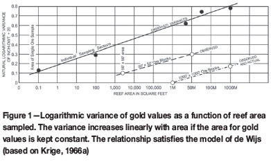
There are two minor departures from the simple model of Equation [2]. The first of these departures is that a small constant term (+20 inch-pennyweights) was added to all gold values. This reflects the fact that, in general, the three-parameter lognormal model provides a better fit than the two-parameter lognormal (Krige, 1960). As will be discussed in more detail later in this paper, this departure corresponds to a narrow secondary peak near the origin of the normal Gaussian frequency density curve for logarithmically transformed gold assay values, and can be explained by adopting an accelerated dispersion model. The second departure consists of the occurrence of constant terms that are contained in the observed logarithmic variances plotted in Figure 1. These additive terms are related to shape differences of the blocks with volumes v and V, as will also be discussed later in this paper.

Worldwide uranium resources

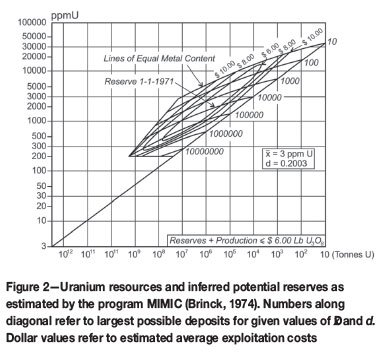
A second example of application of the model of de Wijs is as follows. The log-binomial frequency distribution model was used in mineral resource evaluation studies by Brinck (1971, 1974). A comprehensive review of Brinck's approach can be found in Harris (1984). The original discrete model of de Wijs was assumed to apply to a chemical element in a very large block consisting of the upper part of the Earth's crust with known average concentration value ξ, commonly set equal to the element's crustal abundance or 'Clarke'.

Chemical analysis is applied to blocks of rock that are very small in comparison to the large block targeted for study. Let n = N represent the maximum number of subdivisions of this very large block. Suppose that the element concentration values available for study: (1) constitute a random sample from the population of 2^N small blocks within the large block, and (2) show an approximate straight line pattern on their lognormal Q-Q plot. The slope of this line then provides an estimate of σfrom which η(and d) can be derived by means of the original variance formula of de Wijs. Brinck (1974) set 2^N equal to average weight of the small block used for chemical analysis divided by total weight of the environment targeted for study.

Figure 2 (modified from Brinck, 1974) is a worldwide synthetic diagram for uranium with average crustal abundance value set equal to 3 ppm and dispersion index d = 0.2003. This diagram is equivalent to a cumulative frequency distribution plot with two logarithmic scales. Value (ppm U) is plotted in the vertical direction and weight (tons U) is plotted in the horizontal direction. All weight values are based on cumulative frequencies calculated for the log-binomial distribution and are fully determined by the mean and coefficient of dispersion. The diagram shows curved lines of equal metal content. In 1971 it was, on the whole, profitable to mine uranium if the cost of exploitation was less than US$6.00 per pound U₃O₈. Individual orebodies can be plotted as points in Figure 2. In 1971 such deposits would have been mineable if their point fell within the elliptical contour labeled $6.00. The other elliptical contours are for uranium deposits that would have been more expensive to mine.

 

 

Frequency distributions and spatial statistics

Multiplicative cascade processes that generate spatial frequency distributions of chemical concentration were preceded by generating process models, as will be discussed next.

Theory of proportionate effect

The theory of proportionate effect was originally formulated by Kapteyn (1903) and later in a more rigorous manner by Kolmogorov (1941). It can be regarded as another type of application of the central limit theorem of mathematical statistics. Suppose that a random variable X was generated stepwise by means of a process that started from a constant value X₀. At the i-th step of this process (i = 1, 2, ..., n) the variable was subject to a random change that was a proportion of some function g(X_i-1), or X_i- X_i-1 = ε_i. g(X_i-1). Two special cases are g(X_i-1)= 1 and g(X_i-1)= X_i-1. If g remains constant, X becomes normal (Gaussian) because of the central limit theorem. In the second case, it follows that:

This generating process has the lognormal distribution as its end product. There is an obvious similarity between generating processes and the multiplicative cascade processes to be discussed later in this paper in the context of fractals and multifractals.

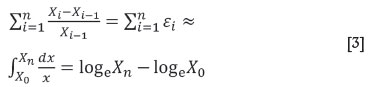
The starting point of the preceding discussion of the generating process also can be written as dX_i= g(X_i).ε_i, where dX_i represents the difference X_i- X_i-1in infinitesimal form. Often an observed frequency distribution can be reduced to normal (Gaussian) form. In Figure 3 a lognormal curve is plotted on normal probability paper. An auxiliary variable z is plotted along the horizontal axis. It has the same arithmetic scale as x, which is plotted in the vertical direction. The variable x is a function of z or x = G(z). The slope of G(z) is measured at a number of points giving the angle φ. For example, if z = x = 20 in Figure 3A, φ= φ₁, and:

 

 

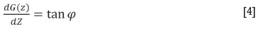
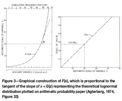
If, in a new diagram (Figure 3B), tan φis plotted against x, we obtain a function F(x) that represents g(X_i) except for a multiplicative constant which remains unknown. This procedure is based on the general solution of the generating process that can be formulated as:

under the assumption that Z is normally distributed.

The function g(X_i)derived in Figure 3B for the lognormal curve of Figure 3A is simply a straight line through the origin. This result is in accordance with the origin theory of proportional effect. However, the method can produce interesting results in situations where the frequency distribution is not lognormal. Two examples are given in Figure 4. The original curves for these two examples (Figure 3) are on logarithmic probability paper. They are for a set of 1000 Merriespruit gold values from Krige (1960), and a set of 84 copper concentration values for sulphide deposits that surround the Muskox intrusion, District of Mackenzie, northern Canada (Agterberg, 1974) as a rim. The results obtained by the graphical method are shown in Figure 4B.

The generating function g(X_i) for Merriespruit is according to a straight line, the extension of which would intersect the X-axis at a point with negative abscissa α= ≈ 55. This is equal to the constant added to pennyweight values by Krige (1960). Addition of this small constant term (55 inch-dwt) to all Merriespruit gold assays has the effect that the straight line in Figure 4B passes through the origin. The departure from lognormality is restricted to the occurrence of a small secondary peak near the origin. The second example (Muskox sulphides) gives a function g(X_i) that resembles a broken line. It would suggest a rather abrupt change in the generating process for copper concentration after the value X_i= ≈ 0.5%. The influence of X_ion dX_i may have decreased with increasing X_i.

The usefulness of a graphical method of this type is limited, in particular because random fluctuations in the original frequency histograms cannot be considered carefully. However, the method is rapid and offers suggestions with respect to the physicochemical processes that may underlie a frequency distribution of observed element concentration values.

Accelerated dispersion model

The model of de Wijs has the property of self-similarity or scale-independence. In his application of this model to gold in the Klerksdorp goldfield, Krige (1966a) worked with approximately 75 000 gold determinations for very small blocks. In Figure 1 it was illustrated that there are approximate straight line relationships between logarithmic variance and logarithmically transformed size of reef area for gold. Validity of the concept of self-similarity was also illustrated by means of moving-average gold value contour maps for square areas measuring 500 ft and 10 000 ft on a side. The contours of moving-average values obtained by Krige (1966a) for these squares show similar patterns of gold concentration contours in both areas, although one area is 400 times as large as the other.

The original assay values satisfy a three-parameter lognormal distribution, because of which a small value was added to all assays to obtain approximate (two-parameter) lognormality. Originally, the following variant of the model of de Wijs was developed (Agterberg, 2007b) because, in a number of applications of the lognormal in resource studies, the high-value tail of the frequency distribution was found to be thicker and longer than log-binomial and lognormal tails. Suppose that the coefficient of dispersion (d) in the model of de Wijs increases as follows with block concentration value (x):

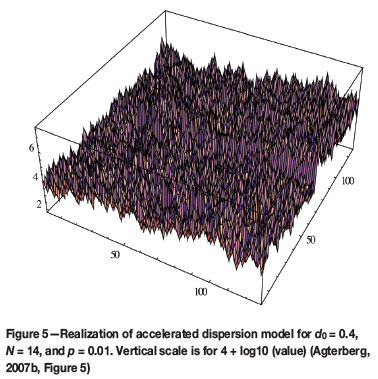
where d₀ represents the initial dispersion index at the beginning of the process, and b is a constant. This accelerated dispersion model produces thicker and longer tails than the lognormal frequency distribution (Agterberg, 2007b). Additionally, it yields more very small values, thus producing a secondary peak near the origin of the frequency density function similar to Merriespruit.

Figure 5 is the result of a two-dimensional computer simulation experiment with d₀= 0.4, n = 14, and p = 0.01. In total, 2¹⁴ = 16 384 values were generated on a 128 x 128 grid. The generating process commenced with a single square with element concentration value set equal to 1. This square was divided into four quadrants of equal size with values (1+d)², (1+d)(1-d), (1-d)(1+d), and (1-d)² in a random configuration (Agterberg, 2001). The process was repeated for each square until the pattern of Figure 5 was obtained. Because p is small, most element concentration values after 14 iterations are nearly equal to values that satisfy the original model of de Wijs. Exceptions are that the largest values, which include (1+d)¹⁴= 316, significantly exceed values that would be generated by the original model, which include (1+d₀)¹⁴= 111 (cf. Agterberg, 2007b, Figure 6). Likewise, the frequencies of very small values that are generated exceed those generated by the ordinary model of de Wijs.

 

 

 

 

Sill and nugget effect

Geostatistical studies are commonly based on a semivariogram fitted to element concentration values from a larger neighbourhood. Generally, these models assume the existence of a 'nugget effect' at the origin, and a 'range' of significant spatial autocorrelation with a 'sill' that corresponds to the variance with respect to regional mean concentration value (see e.g. Journel and Huijbregts, 1978, or Cressie, 1991). It is well known that the 'nugget effect' is generally much larger than chemical determination errors or microscopic randomness associated with ore grain boundaries. This second source of randomness arises because chemical elements are generally confined to crystals with boundaries that introduce randomness at very small scales. In general, the preceding two sources of local randomness have effects that rapidly decline with distance.

Suppose y(h) represents the semivariogram, which is half the variance of the difference between values separated by lag distance h. Semivariogram values normally increase when h is increased until a sill is reached for large distances. If element concentration values are subject to second-order stationarity, y(h) = σ²·(1- p_h)where σ²represents variance and p_his the autocorrelation function. The sill is reached when there is no spatial autocorrelation or y(h) = σ². If regional trends can be separately fitted to element concentration values, the residuals from the resulting regional, systematic variation may become second-order stationary because the overall mean in the study area then is artificially set equal to zero. In most rock types such as granite or sandstone, randomness of chemical concentration is largely restricted to the microscopic scale and sills for compositional data are reached over very short distances. The nugget effect occurs when extrapolation of y(h) towards the origin (h→0) from observed element concentration values yields estimates with y(h) > 0 (or p_h< 1). Often, what seems to be a nugget effect arises when there is strong local autocorrelation that cannot be detected because the locations of samples subjected to chemical analysis are too far apart to describe local continuity.

Matheron (1989) has pointed out that in rock sampling there are two possible infinities if the number of samples is increased indefinitely: either the sampling interval is kept constant so that more rock is covered, or the size of the study area is kept constant whereby sampling interval is decreased. These two possible sampling schemes provide additional information on sample neighbourhood, for sill and nugget effect respectively. In practice, the exact form of the nugget effect usually remains unknown, because extensive sampling would be needed at a scale that exceeds microscopic scale but is less than scale of sampling space commonly used for ore deposits or other geological bodies.

If the model of de Wijs would remain applicable for n →∞, the variance would not exist and it would not be possible to estimate the spatial covariance function. This was the main reason that Matheron (1962, 1989) originally advocated using the variogram, because this tool is based on differences between values that are distance h apart and the existence of a finite variance is not required. Independent of Matheron, Jowett (1955) also advocated use of the variogram instead of the correlogram. Recently, Serra (2014) has calculated the rather strong bias that could result from estimating the spatial covariance from data for which the variance does not exist. Such an approach differs from statistical applications of time series analysis, in which the existence of mean and variance is normally taken for granted. If the variance σ²of spatial observations exists, it follows immediately that the semivariogram satisfies γ_h= σ²- σ_h where σ_h is the covariance of values that are distance h apart. On the other hand, Matheron (1962) originally assumed γ_h= 3A-ln h for logarithmically transformed element concentration values for infinitesimally small volumes, and his approach was in accordance with the model of de Wijs.

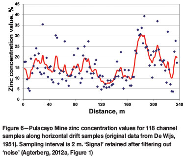
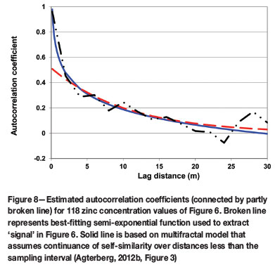
De Wijs (1951) used a series of 118 zinc assays for channel samples taken at 2 m intervals along a drift in the Pulacayo Mine, Bolivia, as an example to illustrate his original model. Matheron (1962) analysed this data-set as well, constructing a semivariogram for the channel samples based on the _γh= 3A. ln h model with _γ0= 0 and σ²= ∞. The original zinc assays for this example are shown in Figure 6. In Agterberg (1974), a standard time series approach was taken in which mean and variance were assumed to exist. The model used for smoothing the 118 zinc values was that each zinc value is the sum of a 'signal' value and small-scale 'noise' with autocorrelation function ρh = c.exp(-ah), where c represents the small-scale noise variance and the parameter a controls the decreasing influence of observed values on their surroundings. The two parameters were estimated to be c = 0.5157 and a = 0.1892. Signal+noise models of this type are well known in several branches of science (cf. Yaglom, 1962). Filtering out the noise component produces the signal shown in Figure 6. Various other statistical methods such as ordinary kriging can be used to produce similar smoothed patterns.

If the logarithmic variance of element concentration values is relatively large, it may not be easy to obtain reliable estimates of statistics such as mean, variance, autocorrelation function, and semivariogram by using untransformed element concentration values. This is a good reason for using logarithmically transformed values instead of original values in such situations. Approximate lognormality for the frequency distribution of element concentration values can often be assumed. If the coefficient of variation, which is equal to the standard deviation divided by the mean, is relatively small (< 0.5), the lognormal distribution can be approximated by a normal (Gaussian) distribution and statistics such as the autocorrelation function can be based on original data without use of a logarithmic transformation. Agterberg (2012a) showed that the estimated and theoretical autocorrelation coefficients for the 118 zinc values from the Pulacayo orebody are almost exactly the same whether or not a logarithmic transformation is used. Consequently, the original data can be used in subsequent statistical calculations for this example.

 

Multifractals

Fractals are objects or features characterized by a fractal dimension that is either greater than or less than the integer Euclidean dimension of the space in which the fractal is embedded. The term 'fractal' was coined by Mandelbrot (1975). On the one hand, fractals are often closely associated with the random variables studied in mathematical statistics; on the other hand, they are connected with the concept of 'chaos' that is an outcome of some types of nonlinear processes. Evertsz and Mandelbrot (1992) explain that fractals are phenomena measured in terms of their presence or absence in cells or boxes belonging to arrays superimposed on the one-, two-, or three-dimensional domain of study, whereas multifractals apply to 'measures' of how much of a feature is present within the cells. Multifractals are either spatially intertwined fractals (cf. Stanley and Meakin, 1988) or mixtures of fractals in spatially distinct line segments, areas, or volumes that are combined with one another. Fractals and multifractals often indicate the existence of self-similarity that normally results in power-law relations (Korvin, 1992; Agterberg, 1995), which plot as straight lines on log-log paper.

Brinck's (1974) model constituted an early application of the model of de Wijs. Estimation of parameters in this model, including d, could be improved by adopting a multifractal modelling approach (Agterberg, 2007a). At first glance, the Brinck approach seems to run counter to the fact that mineral deposits are of many different types and result from different genetic processes. However, Mandelbrot (1983) has shown that, for example, mountainous landscapes can be modeled as fractals. Smoothed contours of elevation on such maps continue to exhibit similar shapes when the scale is enlarged, as in Krige's (1966a) example for Klerksdorp gold contours. Lovejoy and Schertzer (2007) argued convincingly that the Earth's topography can be modelled as a multifractal, both on continents and ocean floors, in accordance with power-law relations originally established by Vening Meinesz (1964). These broad-scale approaches to the nature of topography also seem to run counter to the fact that landscapes are of many different types and result from different genetic processes. In this paper it is assumed that chemical elements within the Earth's crust or within smaller, better-defined environments like the Witwatersrand goldfields can be modeled as multifractals.

The model of de Wijs is a simple example of a binomial multiplicative cascade (cf. Mandelbrot, 1989). Cascade theory has been developed extensively over the past 25 years; for example, by Lovejoy and Schertzer (1991) and other geophysicists (Lovejoy et al., 2010), particularly in connection with cloud formation and rainfall (Schertzer and Lovejoy, 1987; Veneziano and Langousis, 2005). More recently, multifractal modelling of solid Earth processes, including the genesis of ore deposits, has been advanced by Cheng and others (Cheng, 1994, 2008, 2012; Cheng and Agterberg, 1996). In applications concerned with turbulence, the original binomial model of de Wijs became widely known as the binomial/p model (Schertzer et al., 1997). With respect to the problem that in various applications observed frequency distribution tails are thicker than log-binomial or lognormal, it is noted here that several advanced cascade models in meteorology (Veneziano and Langousis, 2005) result in frequency distributions that resemble the lognormal but have thicker tails.

Binomial/p model

The theory of the binomial/p model is clearly presented in textbooks, including Feder (1988), Evertsz and Mandelbrot (1992), Mandelbrot (1989), and Falconer (2003). There have been numerous successful applications of this relatively simple model, including many for solving solid Earth problems (e.g. Cheng, 1994; Cheng and Agterberg, 1996; Agterberg, 2007a,b; Cheng, 2008). Although various departures from the model have also been described in these papers and elsewhere, the binomial/p model remains useful. Basically, it is characterized by a single parameter. In the original model of de Wijs (1951), this parameter is the dispersion index d. When the parameter p of the binomial/p model is used, p = 0.5(1-dh).

Evertsz and Mandelbrot (1992) defined the 'coarse' Hölder exponent αas:

where μrepresents a quantity measured for a cell with volume B_x(∈) around a point x, and ∈ is a line segment, e.g. the edge of cubical cells used to partition the domain of study in a three-dimensional application. In most applications by physicists and chemists, αis called the 'singularity'. The mass-partition function χ_q (∈) is defined as:

where q is a real number (-∞≤ q ≤∞), N(∈)is total number of cells, and N∈ (α) = ∈ -f(α); f(α)represents the fractal dimension for all cells with singularity α. It follows that

At the extremum, for any 'moment' q: and (cf. Evertsz and Mandelbrot, 1992, Equation B.14). Mass exponents τ(q)are defined as:

It follows that , and the so-called multifractal spectrum satisfies:

The preceding derivation is used in the method of moments to construct a multifractal spectrum in practice. This spectrum shows the fractal dimension f(α) as a function of the singularity a and has its maximum f(α) < 1 at α= 1, and f(α)= 0 at two points along the α-axis with:

A one-dimensional example of a multifractal is as follows. Suppose that μ= x. ∈represents the total amount of a metal for a rod-shaped sample that can be approximated by a line segment of length ∈, and x is the metal's concentration value. In the multifractal model it is assumed that (1) μ∞∈∞where ∞denotes proportionality and αis the singularity exponent corresponding to element concentration value x; and (2) N_α(∈) ∞∈^-f(α) represents the total number of line segments of length ∈with concentration value x, while f(α) is the fractal dimension of these line segments.

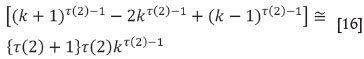
The binomial/p model can be characterized by the second-order mass exponent τ(2) with

If the binomial/p model is satisfied, any one of the parameters p, d, τ(2), α_min, α_max, or σ2 (ln X) can be used for its characterization. Using different parameters can be helpful for checking goodness of fit for the model or finding significant departures from model validity. The mass-partition function and multifractal spectrum of the Pulacayo zinc values were derived by Cheng (1994; also see Cheng and Agterberg, 1996, Figure 2). The line for the second-order moment q = 2 is shown in Figure 7. This line was fitted by least-squares. Its slope provides the fairly precise estimate τ(2) = 0.979 ± 0.038. The degree of fit in Figure 7 is slightly better than can be obtained by semivariogram or correlogram modelling applied to the same data. From this estimate of τ(2) it would follow that d = 0.121.

 

 

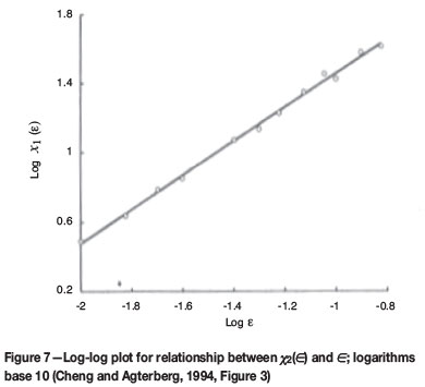
Estimates of a_min and a_max derived for the Pulacayo zinc deposit in Chen et al. (2007) by a technique called 'local singularity analysis' (see later) were 0.532 and 1.697, respectively. Using a slightly different method, Agterberg (2012a) obtained 0.523 and 1.719. These results, which correspond to d = 0.392 Agterberg, 2012b), differ greatly from the estimates based on the binomial/p model with d = 0.121. Clearly, the binomial/p model has a limited range of applicability, although it shows well-defined linear patterns for different moments (q) on the log-log plot of partition function versus ∈(see e.g. Figure 7).

This discrepancy can be explained By using more flexible models with additional parameters, such as the accelerated dispersion model of Equation [6]. The multifractal spectrum resulting from an accelerated dispersion model would be approximately equal to that for the binomial/p model except at the largest (and smallest) concentration values. Because these extreme values occur rarely in practical applications, it follows that the smallest (and largest) singularities that correspond to the extremes cannot be determined by means of the method of moments, which requires relatively large sample sizes. Local singularity analysis has the advantage that it operates on all values from within relatively small neighbourhoods in the immediate vicinity of the extreme values. Another approach resulting in thicker tails is provided by the 'universal multifractal model' initially developed during the late 1990s by Schertzer and Lovejoy (1991). These authors have successfully applied their model to the Pulacayo zinc deposit (Lovejoy and Schertzer, 2007). A basic tool in their approach is the 'first-order structure function', which can be regarded as a generalization of the semivariogram, because differences between spatially separated element concentration values are not only raised to the power 2 but to any positive real number.

Multifractal spatial correlation

Cheng (1994) (also see Cheng and Agterberg, 1996) derived general equations for the semivariogram, spatial covariance, and correlogram of any scale-independent multifractal including the model of de Wijs. Cheng's model is applicable to sequences of adjoining blocks along a line. Experimentally, the resulting semivariogram resembles Matheron's semivar-iogram for infinitesimally small blocks. In both approaches, extrapolation of the spatial covariance function to infinites-imally small blocks yields infinitely large variance when h approaches zero. The autocorrelation function along a line through a multifractal is:

where C is a constant, ∈represents the length of line segment for which the measured zinc concentration value is assumed to be representative, τ(2) is the second-order mass exponent, ξrepresents overall mean concentration value, and σ²(∈) is the variance of the zinc concentration values. The unit interval ∈is measured in the same direction as the lag distance h. The index k is an integer value that can be transformed into a measure of distance by setting k = ½h. Estimation for the 118 Pulacayo zinc values using an ordinary least-squares model after setting τ(2) = 0.979 gave:

The first 15 values (k>1) resulting from this equation are nearly the same as the best-fitting semi-exponential (broken line in Figure 8). This semi-exponential function was used for the filtering in Figure 6. The heavy line in Figure 8 is based on the assumption of scale-independence over shorter distances (h < 2m). It represents a multifractal autocorrelation function.

 

 

This model can be used for extrapolation toward the origin by replacing the second-order difference on the right side of Equation [15] by the second derivative (cf. Agterberg, 2012a, Equation 9):

The theoretical autocovariance function shown as a solid line in Figure 8 was derived by application of this method to lag distances with 2 m > h > 0.014 m. It is approximately in accordance with Matheron's original semivariogram for the Pulacayo zinc assays. For integer values (1 < k < 15), the curve of Figure 7 (solid line) reproduces the estimated autocorrelation coefficients obtained by the original multifractal model using Equation [15]. This method cannot be used when the lag distance becomes very small (h < 0.07 in Figure 8), so that the white noise variance at the origin ( h = 0) cannot be estimated by this method. However, as will be illustrated in the next section, white noise as estimated by local singularity mapping represents only about 2% of the total variability of the zinc values (Agterberg, 2012a). This white noise would represent measurement error and strong decorrelation at microscopic scale.

Singularity analysis

Cheng (1999, 2005) proposed a new model for incorporating spatial association and singularity in interpolation of exploratory data. In his approach, geochemical or other data collected at sampling points within a study area is subjected to two treatments. The first of these is the construction of a contour map by any of the methods, such as kriging or inverse distance weighting techniques, generally used for this purpose. Secondly, the same data is subjected to local singularity mapping. The local singularity αis then used to enhance the contour map by multiplication of the contour value by the factor ∈^α-2where ∈< 1 represents a length measure. In Cheng's (2005) approach to predictive mapping, the factor ∈^a-2 is greater than 2 in places where there has been local element enrichment, or by less than 2 where there has been local depletion. Local singularity mapping can be useful for the detection of geochemical anomalies characterized by local enrichment (cf. Cheng, 2007, Cheng and Agterberg, 2009).

According to Chen et al. (2007), local scaling behaviour follows the following power-law relationship:

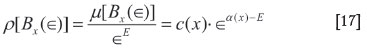
where p{B_x(∈)}represents the element concentration value determined on a neighbourhood size measure B_x at point x, μ(B_x(∈)} represents the amount of metal, and E is the Euclidean dimension of the sampling space. For our 1-dimensional Pulacayo example, E = 1; and, for ∈= 1, B_x extends ∈/2 = 1 m in two directions from each of the 118 points along the line parallel to the mining drift. Suppose that average concentration values p{B_x(∈)}are also obtained for ∈= 3, 5, 7, and 9, by enlarging B_x on both sides. The yardsticks ∈can be normalized by dividing the average concentration values by their largest length (= 9). Reflection of the series of 118 points around its first and last points can be performed to acquire approximate average values of p{B_x(∈)} at the first and last four points of the series. Provided that the model of Equation [17] is valid, a straight line fitted by least squares to the five values of ln μ{B_x(∈)} against a(x).ln ∈then provides estimates of both ln c(x) and α(x) at each point. Chen et al. (2007) proposed an iterative algorithm to obtain improved estimates. Their rationale for this was as follows.

In general, p{B_x(ε)} is an average value of element concentration values for smaller B values at points near x with different local singularities. Consequently, use of Equation [17} would produce biased estimates of c(x) and α(x). How could we obtain estimates of c(x) that are non-singular in that they are not affected by the differences between local singularities within B_x? Chen et al. (2007) proposed to replace Equation. [17] by:

where α*(x) and c*(x) are the optimum singularity index and local element concentration coefficient, respectively. The initial crude estimate c(x) obtained by Equation [17] at step k = 1 is refined repeatedly by using the iterative procedure:

In their application to the 118 zinc values from the Pulacayo orebody, Chen et al. (2007) selected α* (x) = α₄(x) because at this point the rate of convergence has slowed considerably. Agterberg (2012a) duplicated their results and continued the algorithm until full convergence was reached at approximately k = 1000. A bias may arise due to the fact that, at each step of the iterative process, straight-line fitting is being applied to logarithmically transformed variables and results are converted back to the original data scale. This bias can be avoided by forcing the mean to remain equal to 15.61% Zn during all steps of the iterative process. After convergence, all c_k became approximately equal to the average zinc value (= 15.61%). For increasing value of k, c_k represents element concentration values of increasingly large volumes. On the other hand, the corresponding a_k (x) values are singularities for increasingly small volumes around the points x.

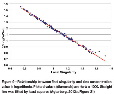
The end product of this application consisted of 118 singularities that are related to the original zinc values according to a logarithmic relationship (Figure 9). It can be assumed that every original zinc value (shown as a cross in Figure 6) is the sum of a true zinc concentration value and an uncorrelated random variable. The latter is a white noise component that would represent both measurement error and strictly local decorrelation because of granularity at the microscopic level. In Figure 9 it is represented by the deviations between the logarithmically transformed measured zinc concentration values and the final singularities obtained at the end of the iterative process. The white noise variance (2.08% of total variance of Zn values) is much smaller than the nugget effect previously used for filtering, which had 48.43% of the total variance.

 

 

Relations between variances for blocks of different sizes and shapes

The following argument is summarized from Agterberg (1984), where further discussions can be found. It is relevant because it is based on the assumption of permanence of shape of frequency distributions of measures on blocks of different sizes. Suppose that a rock or geological environment is sampled by randomly superimposing on it a large block with average value X₂, and that a small block with value X₁ is sampled at random from within the large block. Then the expected value of X₁ is X₂, or E(X₁| X₂) = X₂. Let f(x₁)and f(x₂) represent the frequency density functions of the random variables X₁and X₂, respectively. Suppose that X₁can be transformed into Z₁ and X₂ into Z₂ so that the random variables Z₁ with marginal density function f(z₁), and Z₂ with f(z₂) satisfy a bivariate density function of the type

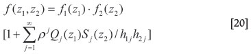
In this equation, ρrepresents the product-moment correlation coefficient of Z₁ and Z₂. Q_j (z₁)and S_j (z₂) are orthogonal polynomials with f₁ and f₂ (z₂) as weighting functions, and with norms h_1j and h_2j respectively. Equation [20] implies

In most applications, f (z₁, z₂) is symmetric with f₁ (zi)= f₂(zi) for f = 1, 2. For example, if f₁ (z₁) and f₂(z₂) are standard normal, Q_j(z₁) = Q_j(z₁) and S_j(z₂) = H_j(z₂) are Hermite polynomials. Then Equation [20] is the Mehler identity, which is well known in mathematics.

When f(x₁) is known, f(x₂) can be derived from Equation [20] in combination with E(X₁ | X₂) = X₂. If f(x₁), and f(x₂) are of the same type, their frequency distribution is called 'permanent'. Six types of permanent frequency distributions are listed in Agterberg (1984). His Type 2 (logarithmic transformation) includes the lognormal and log-binomial distributions. Permanence of these two distributions was first established by Matheron (1974). It means that blocks of different sizes have the same type of frequency distribution; for example, all can be lognormal with the same mean but different logarithmic variances.

It is noted that E(X₁|X₂) = X₂, which can be called the 'regression' of X₁ on X₂, results in the following two relations between block variances:

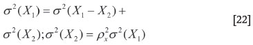
with p_x> 0 representing the product-moment correlation coefficient of X₁and X₂. The first part of Equation [7] can be rewritten as σ²(v, V) = σ²(v) + σ²(V). Suppose that v is contained within a larger volume v that, in turn, is contained within V. Then: σ²(v, V) = σ²(v, V') + σ²(v', V). Equations [20]-[22] are general in that they do not apply only to original element concentration, but also to transformed concentration values; for example, E(ln X₁|ln X₂) = ln X₂.

As mentioned before, Matheron (1962) showed that the semivariogram γ(h) in his extension of the model of de Wijs satisfies γ(h) = 3A.ln h where A is absolute dispersion. This result applies to element concentration values of infinitesimally small blocks at points that are distance h apart. Extending this to volumes v and V by integration yields σ2 (ln x) = A.ln V/v. Suppose that σ2 (v, V) = σ2 (v, V') + σ2 (v', V)applies to volumes v that differ in shape from the volumes v' and V, which have similar shapes. Then Matheron's extension of the model of de Wijs yields: σ2 (v, v') = A.ln (v' /v) + C where C is a constant (cf. Matheron, 1962, Equation IV-57, p. 76). In the application to Witwatersrand gold values there is a distinct shape difference between the linear samples used for assaying and the larger plate-shaped volumes on which the average values were based. This shape difference probably accounts for a constant term included in the observed variances for samples plotted. This constant term (called the 'sampling error' by Krige, 1966a), which equals 0.10 units along the vertical scale in Figure 1) is independent of the size of the area.

 

Concluding remarks

In this paper, Krige's formula for the propagation of metal concentration variances in blocks with different volumes, as well as his demonstration of approximate scale independence of gold assays in the Klerksdorp goldfield, were viewed in the context of multifractal theory. The original model of de Wijs used by Krige and Matheron was the first example of a multiplicative cascade. Various new modifications of this model were discussed to explain inconsistencies that may arise in applications. It was shown that singularity analysis provides useful new information on element concentration variability over distances that are shorter than the sampling intervals used in practice. These new developments reinforce the practical usefulness of Krige's original ideas on self-similarity and scale-independence of patterns of block averages for gold and uranium values in the Witwatersrand goldfields. This paper was mainly a review of recent multifractal theory, which throws new light on the original findings by Professor Danie Krige on self-similarity of gold and uranium patterns at different scales for blocks of ore by (a) generalizing the original model of de Wijs; (b) using the accelerated dispersion model to explain the appearance of a third parameter in the lognormal distribution of Witwatersrand gold determinations; and (c) considering that Krige's sampling error is caused by geometrical differences between single ore sections and reef areas.

 

Acknowledgement

Thanks are due to Dr Zhijun Cheng and two anonymous reviewers for helpful comments that improved the paper.

 

References

Agterberg, F.P. 1961. The skew frequency curve of some ore minerals. Geologie en Mijnbouw, vol. 40. pp.149-162.         [ Links ]

Agterberg, F.P. 1963. Value contours and improved regression techniques for ore reserve calculation. Journal of the South African Institute of Mining and Metallurgy, vol. 64. pp. 108-117.         [ Links ]

Agterberg, F.P. 1966. Two-dimensional weighted moving average trend surfaces for ore evaluation. Proceedings of the Symposium on Mathematical Statistics and Computer Applications in Ore Valuation, 7-8 March 1966. South African Institute of Mining and Metallurgy, Johannesburg. pp. 39-45.         [ Links ]

Agterberg, F.P. 1974. Geomathematics. Elsevier, Amsterdam.         [ Links ]

Agterberg, F.P. 1984. Use of spatial analysis in mineral resource estimation. Mathematical Geology, vol. 16, no. 6. pp. 144-158.         [ Links ]

Agterberg, F.P. 1995. Multifractal modeling of the sizes and grades of giant and supergiant deposits. International Geological Reviews, vol. 37. pp. 1-8.         [ Links ]

Agterberg, F.P. 2001. Multifractal simulation of geochemical map patterns. Geologic Modeling and Simulation: Sedimentary Systems. Merriam, D.F. and Davis, J.C. (eds.). Kluwer, New York. pp. 327-346.         [ Links ]

Agterberg, F.P. 2007a. New applications of the model of de Wijs in regional geochemistry. Mathematical Geology, vol. 39, no. 1. pp. 1-26.         [ Links ]

Agterberg, F.P. 2007b. Mixtures of multiplicative cascade models in geochemistry. Nonlinear Processes in Geophysics, vol. 14. pp. 201-209.         [ Links ]

Agterberg, F.P. 2012a. Sampling and analysis of element concentration distribution in rock units and orebodies. Nonlinear Processes in Geophysics, vol. 19. pp. 23-44.         [ Links ]

Agterberg, F.P. 2012b. Multifractals and geostatistics. Journal of Geochemical Exploration, vol. 122. pp. 113-122.         [ Links ]

Brinck, J.W. 1971. MIMIC, the prediction of mineral resources and long-term price trends in the non-ferrous metal mining industry is no longer Utopian. Eurospectra, vol. 10. pp. 46-56.         [ Links ]

Brinck, J.W. 1974. The geochemical distribution of uranium as a primary criterion for the formation of ore deposits. Chemical and Physical Mechanisms in the Formation of Uranium Mineralization, Geochronology, Isotope Geology, and Mineralization. IAEA Proceedings Series STI/PUB/374. pp. 21-32.         [ Links ]

Chen, Z., Cheng, Q., Chen, J., and Xie, S. 2007. A novel iterative approach for mapping local singularities from geochemical data. Nonlinear Processes in Geophysics, vol. 14. pp. 317-324.         [ Links ]

Cheng, Q. 1994. Multifractal modeling and spatial analysis with GIS: gold mineral potential estimation in the Mitchell-Sulphurets area, northwestern British Columbia. Doctoral dissertation, University of Ottawa.         [ Links ]

Cheng, Q. 1999. Multifractality and spatial statistics. Computers and Geosciences, vol. 25. pp. 949-961.         [ Links ]

Cheng, Q. 2005. A new model for incorporating spatial association and singularity in interpolation of exploratory data. Geostatistics Banff 2004. Leuangthong, D. and Deutsch, C.V. (eds.). Springer, Dordrecht, The Netherlands. pp. 1017-1025.         [ Links ]

Cheng, Q. 2007. Mapping singularities with stream sediment geochemical data for prediction of undiscovered mineral deposits in Gejiu, Yunnan Province, China. Ore Geology Reviews, vol. 32. pp. 314-324.         [ Links ]

Cheng, Q. 2008. Non-linear theory and power-law models for information integration and mineral resources quantitative assessments. Progress in Geomathematics. Bonham-Carter, G. and Cheng, Q. (eds.). Springer, Heidelberg. pp. 195-225.         [ Links ]

Cheng, Q. 2012. Multiplicative cascade processes and information integration for predictive mapping. Nonlinear Processes in Geophysics, vol. 19. pp. 1-12.         [ Links ]

Cheng, Q. and Agterberg, F.P. 1996. Multifractal modelling and spatial statistics. Mathematical Geology, vol. 28, no. 1. pp.1-16.         [ Links ]

Cheng, Q. and Agterberg, F.P. 2009. Singularity analysis of ore-mineral and toxic trace elements in stream sediments. Computers and Geosciences, vol. 35. pp. 234-244.         [ Links ]

Cressie, N.A.C. 1991. Statistics for Spatial Data. Wiley, New York.         [ Links ]

De Wijs, H.J. 1948. Statistische methods toegepast op de schatting van ertsreserven. Jaarboek der Mijnbouwkundige Vereniging te Delft, 1947-1948. pp. 53-80.         [ Links ]

De Wijs, H.J. 1951. Statistics of ore distribution. Geologie en Mijnbouw, vol. 30. pp. 365-375.         [ Links ]

Evertsz, C.J.G. and Mandelbrot, B.B. 1992. Multifractal measures. Chaos and Fractals. Peitgen, H.-O., Jurgens, H., and Saupe, D. (eds.). Springer-Verlag, New York.         [ Links ]

Falconer, K. 2003. Fractal Geometry. 2nd edn. Wiley, Chichester.         [ Links ]

Feder, J. 1988. Fractals. Plenum, New York.         [ Links ]

Harris, D.P. 1984. Mineral Resources Appraisal. Clarendon Press, Oxford.         [ Links ]

Journel, A.G. and Huijbregts, C.J. 1978. Mining Geostatistics. Academic Press, New York.         [ Links ]

Jowett, G.H. 1955. Least-squares regression analysis for trend reduced time series. Journal of the Royal Statistical Society, Series B, vol. 17. pp. 91-104.         [ Links ]

Kapteyn, J.C. 1903. Skew Frequency Curves in Biology and Statistics. Noordhoff, Groningen.         [ Links ]

Kolmogorov, A.N. 1941. On the logarithmic normal distribution law for the sizes of splitting particles. Doklady Akademia Nauk SSSR, vol. 31. pp. 99-100.         [ Links ]

Korvin, G. 1992. Fractal Models in the Earth Sciences. Elsevier, Amsterdam.         [ Links ]

Krige, D.G. 1951a. A statistical approach to some mine valuation and allied problems on the Wtwatersrand. MSc thesis, University of the Witwatersrand, Johannesburg.         [ Links ]

Krige, D.G. 1951b. A statistical approach to some basic valuation problems on the Witwatersrand. Journal of the South African Institute of Mining and Metallurgy, vol. 52. pp. 119-139.         [ Links ]

Krige, D.G. 1955. Emploi statistique mathematique dans les problèmes poses par l'éevaluation des gisements. Annales des Mines, Décembre.         [ Links ]

Krige, D.G. 1960. On the departure of ore value distributions from the lognormal model in South African gold mines. Journal of the South African Institute of Mining and Metallurgy, vol. 61. pp. 231-244.         [ Links ]

Krige, D.G. 1966a. A study of gold and uranium distribution pattern in the Klerksdorp goldfield. Geoexploration, vol. 4. pp. 43-53.         [ Links ]

Krige, D.G. 1966b. Two-dimensional weighted moving average trend surfaces for ore valuation. Proceedings of the Symposium on Mathematical Statistics and Computer Applications in Ore Valuation, 7-8 March, 1966. South African Institute of Mining and Metallurgy, Johannesburg. pp. 13-38.         [ Links ]

Krige, D.G. 1978. Lognormal-de Wijsian Geostatistics for Ore Evaluation. Monograph Series, vol.1. South African Institute of Mining and Metallurgy, Johannesburg.         [ Links ]

Krige, D.G. and Ueckermann, H.J. 1963. Value contours and improved regression techniques for ore reserve valuations. Journal of the South African Institute of Mining and Metallurgy, vol. 63. pp. 429-452.         [ Links ]

Lovejoy, S. and Schertzer, D. 1991. Multifractal analysis techniques and the rain and cloud fields from 10-3 to 106 m. Non-linear Variability in Geophysics. Schertzer, D. and Lovejoy, S. (eds.). Kluwer, Dordrecht. pp. 111-144.         [ Links ]

Lovejoy, S. and Schertzer, D. 2007. Scaling and multifractal fields in the solid earth and topography. Nonlinear Processes in Geophysics, vol. 14. pp. 465-502.         [ Links ]

Lovejoy, S., Agterberg, F., Carsteanu, A., Cheng, Q., Davidsen, J., Gaonac'h, H., Gupta, V., l'Heureux, I., Liu, W., Morris, S.W., Sharma, S., Shcherbakov, R., Tarquis, A., Turcotte, D., and Uritsky, V. 2010. Nonlinear geophysics: why we need it. EOS, vol. 90, no. 48. pp. 455-456.         [ Links ]

Mandelbrot, B.B. 1975. Les Objects Fractals: Forme, Hazard et Dimension. Flammarion, Paris.         [ Links ]

Mandelbrot, B.B. 1983. The Fractal Geometry of Nature. Freeman, San Francisco.         [ Links ]

Mandelbrot, B.B. 1989. Multifractal measures, especially for the geophysicist. Pure and Applied Geophysics, vol. 131. pp. 5-42.         [ Links ]

Matheron, G. 1955. Application des methods statistiques à l'évaluation des gisements. Annales des Mines, Décembre.         [ Links ]

Matheron, G. 1962. Traité de géostatistique appliquée. Mémoires de BRGM, 14. Paris.         [ Links ]

Matheron, G. 1967. Kriging or polynomial interpolation procedures? Transactions of the Canadian Institute of Mining and Metallurgy, vol. 70. pp. 240-242.         [ Links ]

Matheron, G. 1974. Les fonctions de transfert des petits panneaux. Note Geostatistique 127. Centre de Morphologie Mathematique, Fontainebleau, France.         [ Links ]

Matheron, G. 1989. Estimating and choosing, an essay on probability in practice. Hasover, A.M. (trans.). Springer, Heidelberg.         [ Links ]

Schertzer, D. and Lovejoy, S. 1987. Physical modeling and analysis of rain and clouds by anisotropic scaling of multiplicative processes. Journal of Geophysical Research, vol. 92. pp. 9693-9714.         [ Links ]

Schertzer, D. and Lovejoy, S. (eds.). 1991. Non-linear Variability in Geophysics. Kluwer, Dordrecht.         [ Links ]

Schertzer, D., Lovejoy, S., Schmitt, F., Chigirinskaya, Y. and Marsan, D. 1997. Multifractal cascade dynamics and turbulent intermittency. Fractals, vol. 5. pp. 427-471.         [ Links ]

Serra, J. 2014 Revisiting 'Estimating and Choosing'. Mathematics of Planet Earth. Pardo-Igúzquiza, E., Guardiola-Albert, C., Heredia, J., Moreno-Merino, L., Durán, J.J., and Vargas-Guzmán, J.A. (ed.). Springer, Heidelberg. pp. 57-60.         [ Links ]

Sichel, H.S. 1952. New methods in the statistical evaluation of mine sampling data. Journal of the South African Institute of Mining and Metallurgy, vol. 61. pp. 261-288.         [ Links ]

Sichel, H.S. 1961. On the departure of ore value distributions from the lognormal model in South African gold mines. Journal of the South African Institute of Mining and Metallurgy, vol. 62. pp. 333-338.         [ Links ]

Stanley, H. and Meakin, P. 1988. Multifractal phenomena in physics and chemistry. Nature, vol. 335. pp. 405-409.         [ Links ]

Veneziano, D. and Langousis, A. 2005. The maximum of multifractal cascades: exact distribution and approximations. Fractals, vol. 13, no. 4. pp. 311-324.         [ Links ]

Vening Meinesz, F.A. 1964. The Earth's Crust and Mantle. Elsevier, Amsterdam.         [ Links ]

Yaglom, A.M. 1962. An Introduction to the Theory of Stationary Random Functions. Prentice-Hall, Englewood Cliffs, NJ.         [ Links ]