On the reduction of algorithmic smoothing of kriged estimates

 

 

L. Tolmay

Sibanye Gold, Johannesburg, South Africa

 

 

---

SYNOPSIS

Utilizing a very large database from a mined-out area on a South African gold mine, the relative efficacy of a method to mitigate the smoothing effect introduced by the algorithmic constraints imposed by kriging was investigated. Smoothing effects arising from limited data availability are differentiated from the smoothing arising from the application of estimation algorithms. Very little can be done to ameliorate smoothing of estimates because of too little data, barring additional drilling or sampling. However, the smoothing effects resulting from the kriging process are shown to be mitigated by use of an alternative algorithm. The primary criterion in the development of the new algorithm was to avoid re-introducing conditional bias. This paper examines firstly the smoothing effects introduced into estimates via the kriging covariance matrix, secondly the process for ameliorating the smoothing effect, and finally it uses a case study to demonstrate the effectiveness of the new algorithm on a very large database. The database was used to introduce a 60 m by 60 m drilling pattern which in turn was used to model the semi-variogram and produce 30 m by 30 m kriged block estimates. The follow-up database was then re-introduced (roughly 5 m by 5 m grid spacing) and averaged into 30 m by 30 m blocks to provide a direct comparison with the initial estimates. In this way the extent of smoothing and accuracy of the estimates before and after the corrections was tested.

Keywords: kriging, smoothing, direct conditioning, kriging weights, algorithmic smoothing.

---

 

 

Introduction

Smoothing of kriged local estimates on an operating mine that uses selective mining is undesirable. Smoothing reduces the resolution of individual estimates, thus inhibiting the selection process and leading to sub-optimal mining practices. Although the overall average grade may be correct, only selected portions of the orebody are mined. Our concern is not with how much pay or unpay ground exists within a certain area, but rather where it exists, and where to drill and blast. The problem is exacerbated on marginal mines, where smoothing obscures small differences in grade and could result in incorrect allocation of pay ground to waste, or vice versa, and lead to substantial financial losses. Although various post-processing techniques are used to correct smoothing, such as spectral post-processor, (Journel et al., 2000), conditional simulations, indirect post-processing techniques (Assibey-Bonsu and Krige, 1999), and localized direct conditioning (Assibey-Bonsu and Krige 1999; Krige, Assibey-Bonsu, and Tolmay, 2008), these have dealt with smoothing as a single phenomenon and not identified algorithmic smoothing on its own. Thus the aim of this research was to devise a methodology that reduces the algorithmic smoothing of individual estimates.

The method has not yet been integrated into the kriging process, but can easily be integrated into the underlying mathematical formalism in the future.

 

Why algorithmic smoothing occurs

In the case of simple kriging, the weight assigned to the mean increases as estimates move further away from the data source, but in the case of ordinary kriging the criterion is that the sum of the weights should add up to unity, and this is exactly the reason for the occurrence of algorithmic smoothing in this case. If relatively few samples are included in the estimation process there are likely to be large differences between weightings. However, as the number of samples used in estimation increases, the differences between weightings decreases until these differences become so small that the weights to all intents and purposes are considered to be equal. At this stage the estimate simply becomes the arithmetic mean of the samples used in the estimate. This effect is demonstrated in Figure 1.

 

 

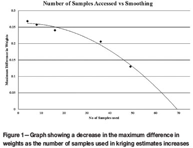
Figure 1 illustrates how the maximum difference in weights decreases as the number of samples used in the kriging estimates increases, in this case the difference being close to zero when approximately 68 samples are used. At this stage the estimate is a totally smoothed estimate of all samples used and will, to all intents and purposes, be equal to the simple arithmetic mean.

 

Methodology

The premise for applying a new methodology is that at least some of the smoothing of kriged estimates is a direct result of the estimation algorithm. The smoothing results in kriged estimates moving toward the mean, the movement being negative if the estimate is above the mean and positive if the estimate is below the mean. The smoothing effect is zero when the distance between the location of the point being estimated and the location of the samples is zero. In addition, if the weight attributable to a sample is zero the smoothing effect on the estimate is also zero. Similar estimation weights result in similar smoothing effects (with the proviso that they are in the same direction and have the same distance); hence the circumstances relevant to an estimate may be different from one estimate to another. This means that in order to obtain an unbiased estimate, the amount by which an estimate must move away from the average value of samples on one side of an estimate is equivalent to the amount by which it must move towards the average value of the samples on the other side of the estimate. Thus any attempt to remove the effects of smoothing must take into account:

> The distance and direction of the sample from the estimate

> The estimation weighting of each sample

> The value of the sample relative to the mean of all samples

> Whether or not the sample used is above or below the average of all samples used

> Each estimate must be considered on its own merit

> The amount by which an estimate must move away from the average value of samples on the one side of an estimate to get to the actual value is equivalent to the amount by which it moves towards the average value on the alternative side of the estimate.

If the kriged estimate is considered to be the best linear unbiased estimate, given the sampling data and the associated semivariogram model, one can reasonably assume that the difference between the estimate and its corresponding actual value is attributable to the smoothing effects of both information and algorithmic. From the basic premises outlined above, the following algorithm represents the proposed solution for a unsmoothed, unbiased value of a kriged estimate:

Substituting SB with 1/SA gives:

Re-arranging and multiplying by SA;

where

WA a kriging weight for a value above the estimate

WB a kriging weight for a value below the estimate

SA the smoothing effect attributable to the sampling above the estimate

SB the smoothing effect attributable to the sampling below the estimate

IA samples used for estimation whose values are above the estimate

IB samples used for estimation whose values are below the estimate

SB 1/SA. This is inferred from the last point in underlying premises above, and is a pre-condition and axiomatic.

Solving Equation [3] provides a correction for the smoothing effect on an individual estimate. For any quadratic equation such as that shown in Equation [3], two solutions exist, one of which is correct and the other extraneous, so due caution must be exercised as only the solution which increases the weighting on the side of the estimate opposite to the smoothing effect will provide a corrected estimate. The point is illustrated in the example presented in Table I.

 

 

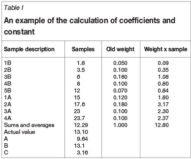
Table I shows the estimated value, 12.80 compared to the actual follow-up value of 13.1. Substituting the coefficients from Table I into Equation [3] yields:

and solving for SA we obtain:

or

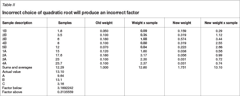
In this case the estimated value must increase in order to move from the estimate to the actual value. Thus the correction factor must increase the weighting of the samples above the estimate and decrease it for those below the estimate. An example of choosing the wrong root as a solution for our quadratic equation is shown in Table II.

As can be observed in Table II, although the correction factor produces the correct value, it does not increase the weights of the samples above the estimate and hence is the extraneous solution. An example of the choice of the correct quadratic root is illustrated in Table III.

In Table III, the selection of the correct quadratic root provides a correction factor that increases the weights of the values above the estimate and is therefore the correct factor.

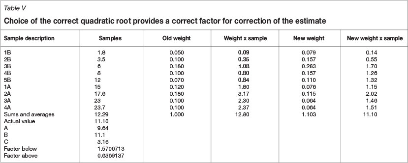
We should now consider the case in which the smoothing has increased the value of the estimate, as shown in Table IV.

 

 

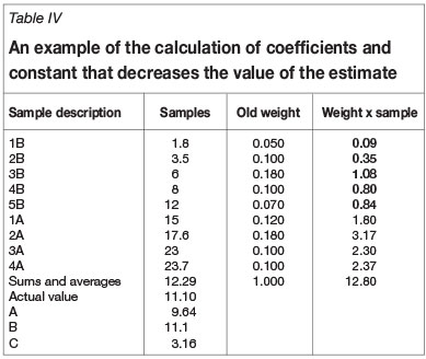
The value of the estimate shown in Table IV is 12.8, whereas the actual follow-up value is 11.1. Again, substituting the appropriate coefficients from Table V gives:

Solving for SA gives:

or

In this case, in order to move from the estimate to the actual value, the value must decrease. Therefore the correction factor must decrease the weighting of samples above the estimate, and increase that of those below the estimate. An example of choosing the correct root as a solution for our quadratic equation in this case is shown in Table V.

As can be observed from Table V, the correction factor produces the correct value, and increases the weights of the samples below the estimate and hence is a valid solution.

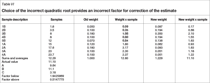
Consider Table VI, where the correction factor increases the weights of the values below the estimate and hence is a valid solution, however not the optimal.

In the second example, shown in Tables V and VI, we are presented with two valid solutions. The choice of which one to use should be based on the rational decision not to reintroduce conditional bias, and it is therefore the solution having the lowest factor for increasing the weights below the mean.

One may ask why smoothing above the estimate was solved for in both cases, rather than above and below. The answer is that under certain conditions when solving for the smoothing below, b2 - 4ac provides a negative value and hence is not solvable; however, this does not occur in the case of solving for the smoothing factor above the estimate. Thus it is possible, using a cross-validation routine, to calculate the smoothing correction for various distances and directions. These can then be modelled and used in a corresponding correction for smoothing routine.

 

The process

The process for reduction of algorithmic smoothing for each estimate with a follow-up actual can be summarized as follows:

> Utilizing the samples used for the estimate, calculate and save the correction factor for each sample distance and direction

> Average the correction factors into directions and distances using a directional and lag tolerance. Although in an entirely homoschedastic environment those correction factors for increasing and decreasing grades of estimates should theoretically be similar, the spatial relationships surrounding these may not be so. It is therefore prudent to model the factors for increasing grade estimates separately from those for decreasing grade estimates

> Model the correction factors

> For each estimate, apply model of correction factors to each sample in order to obtain the corrected weight, taking due cognisance of where the individual sample is in relation to the estimate and the mean of all samples used, i.e.

- If the estimate is below the mean then the smoothing will have dragged the estimate upwards towards the mean. Hence values below the estimate will have a weight correction factor greater than unity, and values above the estimate will have the weight correction factor less than unity

- If the estimate is above the mean then the smoothing will have dragged the estimate downwards towards the mean. In this case values above the estimate will have a weight correction factor greater than unity, whereas those values below the estimate will have the weight correction factor less than unity

> Use the corrected weights to obtain new estimate.

An outstanding question, for which there is no immediate answer, is 'does the kriging variance include the error made in the smoothing of the estimate?' If the answer is yes, as the author suspects is the case, the distribution of errors will no longer be symmetrical around the adjusted estimate and will have to be corrected for by the amount of the adjustment.

 

The case study (or doing it Danie's way)

A sampling database of 61 834 individual channel samples was used for the follow-up. The database used for estimation was obtained by overlaying a 60 by 60 m grid on the channel samples, and using the sample closest to the centre of each 60 by 60 m block as a drill point. In addition, 3 years of data was removed in order to check on the effects of extrapolation as well as interpolation.

Using the abovementioned data a 30 by 30 m grid was kriged and used for the analysis. The follow-up was obtained by utilizing all the data in 30 by 30 m averaged blocks that had a minimum of 14 samples within the block in order to ensure representative means for each block. This methodology was employed to obtain robust, smoothed estimates from a regular grid underlying the area of interest. These estimates were used to reduce the levels of smoothing and to test the efficiency of the newly proposed method, rather than improving the estimates per se. Nevertheless, a certain amount of reduction in error would of necessity be observed due to the averaging process, the results being shown in Table VII.

 

 

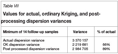
Table VII indicates that the dispersion variance of the adjusted values (post-processed dispersion variance) is improved relative to that of the ordinary kriging, thus rendering a greater resolution of estimates.

A regression plot of the unmodified ordinary kriged estimates can be compared with the modified estimates in Figure 2a and 2b. The unmodified estimates have a multiplicative bias of 1.188, while the modified estimates only show a bias of 1.037. The question as to whether the modified estimates are actually of greater quality must be answered in the affirmative, with only a marginal conditional bias and seemingly less error.

 

 

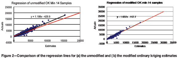
Although a large proportion of the smoothing is removed (Figure 2b compared with Figure 2a), a minor amount of smoothing, reflected as a 1.037 multiplicative bias due to the information effect, remains.

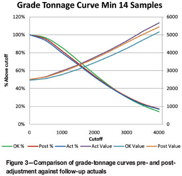
When the data is plotted in grade-tonnage curves as shown in Figure 3, it is evident that the curves for the modified data are closer to the actual curves than the unmodified ordinary kriging estimates.

 

 

Conclusion

Comparison of the modified and unmodified kriging estimates on regression curves and grade-tonnage curves indicates that the newly proposed algorithm for eliminating the effects of algorithmic smoothing through the ordinary kriging process achieves this end in an effective manner without re-introducing conditional bias. This method can be effectively applied in areas with limited sampling coverage, and where the effects of smoothing could adversely impact current and future mining plans.

 

Acknowledgement

To Daniel Gerhardus Krige, for showing me the benefit of plugging along even when it appears that no-one is listening.

 

References

Assibey-Bonsu, W. and Krige, D.G. 1999. Use of direct and indirect distributions of selective mining units for estimation of recoverable resource/reserves for new mining projects. APCOM'99, Proceedings of the 28th International Symposium on Computer Applications in the Minerals Industries, Colorado School of Mines, Golden, CO, 20-22 October 1999.         [ Links ]

Assibey-Bonsu, W., Krige, D.G., and Tolmay, L. 2008. Uncertainty grade assessment for short and medium-term mine planning of underground mining operations. Proceedings of the 8th International Geostatistics Congress, Santiago, Chile, 1-5 December 2008. Ortiz, J.M. and Emery, X. (eds.). pp. 739-748.         [ Links ]

Journel, A.G., Kyriadkidis, P.C., and Mao, S. 2000. Correcting the smoothing effect of estimators: a spectral postprocessor. Mathematical Geology, vol. 32, no. 7. p. 787-813.         [ Links ]

Krige, D.G. 1999. Conditional biases and uncertainty of estimation in geostatistics. APCOM'99, Proceedings of the 28th International Symposium on Computer Applications in the Minerals Industries, Colorado School of Mines, Golden, CO, 20-22 October 1999.         [ Links ]

Matheron, G. 1960. Krigeage d'un Panneau Rectangulaire par sa Peripherie. Note Géostatistique, no. 28.         [ Links ]