Witwatersrand gold reef evaluation: the ‘variancegram’ tool

 

 

C. Lemmer^I; M. Mogilnicki^II

^IGeological and Geostatistical Services, Johannesburg, South Africa
^IIAsfaltowa, Warsaw, Poland

 

 

---

SYNOPSIS

The resolution with which the different categories of resources are forecast for Witwatersrand gold reefs should ideally tie in with block sizes that are optimal in terms of the variability structures of the reefs. A tool, called the 'variancegram', is proposed as a basis for block size choice. A variancegram is intrinsic to the particular reef and mine concerned. A further requirement is the ability to attach global confidence limits to weighted average estimates built up from combinations of local kriged estimates. Approximations to derive global kriging variances based on variables derived from local kriging deliver hugely inflated results if ordinary kriging is used, and markedly better, but not accurate, values if simple kriging is used. These approximations improve as the number of samples used in kriging each block is increased. It is shown that the behaviour of the different components of the global kriging variance with increasing number of samples, all differs, but they all link to the variancegram for the particular reef. The variancegram can thus be used to correct the different components to the values they would have had if all samples were used in kriging each block, and so deliver the 'correct' global kriging variance, even though only a limited number of samples were used in kriging each block. The desirability of having very stable solutions implemented in production systems is taken into account in the proposals. It is anticipated that the same variancegram findings will also hold for other densely sampled deposits, but this remains to be investigated.

Keywords: resources, classification, global kriging variance.

---

 

 

Introduction

The Witwatersrand gold reefs in South Africa are unique in terms of their continuity despite the relatively narrow reef widths. This aspect, together with the wealth of historical channel sample data captured, affords the rare opportunity of studying gold accumulation behaviour over square kilometres in extent. Such studies have in turn provided the backdrop against which large-scale forecasts can be attempted for a phenomenon as inherently variable as gold, and at such extreme mining depths. Due to the latter circumstance, forecasting of values ahead of a mining front is based almost exclusively on extrapolation.

Although the channel sample data itself exhibit very high micro-scale variability (which all but masks any spatial continuity), it is well-known in the industry that, by averaging these data values into blocks of ever-increasing size, one can uncover spatial structures (variograms) with ever-increasing ranges to underpin the extrapolation. This practice serves the needs of the industry: resources within a short range of the just-mined blocks constitute the 'annual forecast' or Measured Resource for the coming year, and need to be estimated with relatively high resolution; resources beyond these constitute 'medium term' or Indicated Resources that may be mined within the following five years, and the resolution requirements for these resources are less stringent; finally, the remaining resources constitute the 'long-term' or 'life-of- mine' or Inferred Resources, and the resolution required for these last estimates is relatively crude.

In choosing the block sizes on which the averaging process will be based, one can be purely practical and choose the block dimension such that the resulting range will cover the area to be estimated. However, one is dealing with a geological phenomenon here, and there is an instinctive feeling that optimum block sizes - in terms of best elucidating the underlying spatial structures -will be peculiar to the reef or deposit studied.

A tool called a 'variancegram' is proposed for determining the underlying optimum block sizes. There is a small latitude in the final determination of the sizes, allowing the very desirable feature of having the block sizes as integer multiples of each other and thus multiples of the smallest block size chosen. This feature forms a cornerstone for the development of an overall gold resource system, and the justification for considering the derived block sizes as 'optimal' will also be discussed.

Having forecast (kriged) the resources remaining to be mined with different degrees of resolution, the associated practical problem of the need for confidence limits to attach to average values built up from combinations of these varying supports is posed. In essence, this boils down to the intractable problem of the inability to derive a global kriging variance by a simple combination of local kriging variances. A first approximation to the problem, which has been mooted in the literature, is discussed.

The quality of the above-mentioned approximation is very dependent on the number of samples used to krige each of the local estimates. Theoretically, if all available samples were used to krige each local estimate, the resultant global kriging variance should be good. However, for most of the practical numbers of samples routinely used in such kriging, the approximation delivers a hugely inflated global kriging variance if ordinary kriging (OK) was done, and a markedly better, but not accurate, value if simple kriging (SK) was carried out.

The interesting finding is that, with increasing numbers of samples, the behaviour patterns of the different components of the global kriging variance, for OK or SK, differ; but they all link to the behaviour of the variancegram for the particular gold reef under consideration.

A method for correcting the above-mentioned inaccurate global kriging variances is proposed, based on the variancegram.

It is anticipated that the same variancegram findings will also hold for other densely sampled deposits, but this remains to be investigated.

 

The variancegram

Early work of Krige, published during the 1950s and summarized later (Krige, 1978), found that 'the logarithmic variance of gold values shows a rising linear trend when plotted against the logarithms of the population areas concerned. This remarkable finding is, of course, true in theory and it would certainly be true for infinite deposits, but in practice one finds that the variance of the logarithms of the gold accumulation values, or logvariance for brevity, does not steadily increase without limit, but that it starts to deflect downwards towards an eventual 'sill'.

For the purposes of determining optimum block sizes - to use in the routine evaluation of gold reefs - it was decided to investigate the above deflection points, with the view that they indicate points at which the logvariance decreases abruptly due to correlations between sample values that set in for areas beyond that particular size. The argument is that by averaging point values within an area indicated by, for instance, the first deflection point, one would absorb the first-structure variability within the block averages, and a variogram in terms of these averages would then elucidate longer-range structures.

Channel sample data (gold accumulation values) for a typical reef was available over several square kilometres in area (the 'test data'). The logvariance of this 'point' test data was calculated within grid cells of side 7 m, 8 m, etc., up to cells of dimension 2000 m, and finally 5000 m. For each choice of cell size the logvariance for that cell size, averaged over the entire mine, was determined.

Figure 1 shows the graph resulting when the average logvariance per cell is plotted against the logarithm of the area of the cell.

 

 

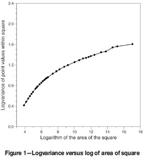
As is clear from this graph, it was found that the series of deflections does not constitute sharp, unique bends. On the contrary, by drawing tangential lines to the graph, several sets of deflection points can be obtained.

A solution to this problem was found by plotting the average logvariance within square cells against the length of the side of the square. Figure 2 shows the resultant graph for the reef under consideration.

 

 

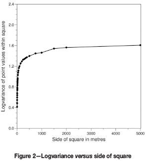
In contrast with Figure 1 this plot uses the effective block (cell) side length to characterize the area under consideration. Such a construction will, for the purpose of this discussion, be called a 'variancegram' to distinguish it from the more familiar variogram of classical geostatistics. The distinction is all the more important since (i) the plot has the appearance of a variogram (which it is not), and (ii) in describing its main features one can draw on previous experience of fitting ordinary variograms. Point (ii) will be discussed in more detail below.

One notices from Figure 2 that the rate at which the logvariance varies with changes from a rapid to a much slower one as the side of the block involved is increased. If the initial rapid variation in the logvariance is interpreted as a reflection of the microstructure variability in the deposit, then this rapid increase in logvariance with block side would be expected to continue without limit as l increases, if this variability persists at all scales. Obviously this does not happen in the case of the test data. Instead, the logvariance increases less and less rapidly as l is increased, and dramatically so.

This empirical finding is to be interpreted as reflecting the presence of a set of superimposed micro-to-macro variability structures in the deposit, each exhibiting a characteristic range a over which it is operative, and beyond which it levels off to a constant value. For block sizes of dimension larger than a, it would lead to a smaller logvariance than would otherwise have been found had the particular structure continued to increase at the same rate for all distances.

The preceding qualitative observation can be made quantitative by drawing on the understanding of the meaning of the spherical model in fitting variograms. As is well-known, the spherical model formula is equivalent to surrounding each point grade by a 'sphere of influence' with radius equal to one-half the variogram range a, and arguing that the covariance of two grades at positions separated by h < a is proportional to the overlap volume of their respective spheres of influence. This assumption immediately gives

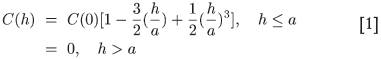
for the covariance, from which the standard spherical variogram formula follows,

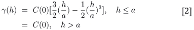
i.e. the variogram is proportional to the non-overlapping volume, and when the two spheres are separated by a distance of more than a, the non-overlapping volume has reached a constant value.

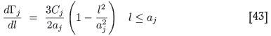
These ideas can now be taken over to provide the basis for a quantitative method for describing the variancegram as well. For, by analogy with the variogram case, one can argue that the variability associated with a structure of range a in the deposit increases with square side l within a 'sphere of influence' of radius a, beyond which the variability levels off once l exceeds a. Then it immediately follows that the logvariance (due to all structures present), as a function of increasing square size, will gradually start to saturate as it approaches a final value, instead of increasing indefinitely. Calling the variancegram Γ(l) to carefully distinguish it from the usual variogram, one can write

for the influence of the ith structure in the variancegram. The variancegram itself is then constructed as follows:

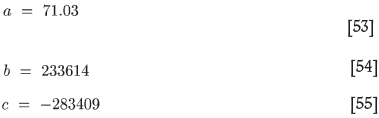
It is to be emphasized again that this is a parametrization of the variancegram that has been motivated by ideas suggested by the meaning of correlation in the case of the ordinary variogram. The big advantage of the approach is that one draws on existing expertise and programs to fit the curve.

In fitting the test data, it turned out that the spherical model gives an extremely good representation of the empirical variancegram. Figure 3 shows the experimental data points, with the model fitted.

 

 

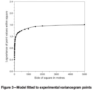
The parameters of the fitted model are the following (using the standard spherical model notation):

C₀ = 0

C1 = 0.710, a₁ = 20 m

C₂ = 0.280, a₂ = 60 m

C₃ = 0.190, a₃ = 180 m

C₄ = 0.118, a₄ = 540 m

C₅ = 0.205, a₅ = 1620 m

C₆ = 0.097, a₆ = 4860 m

The advantage of fitting a nested spherical model is that it fits a continuous curve, even though there are six structures. There is thus no need to try to divine successive bends in the experimental curve.

In establishing a good fit, there is a small amount of latitude in choosing the 'sills' C and the ranges a. However, the systematic increase in the ranges is no doubt an intrinsic property of the variability structures of the deposit, and arbitrarily chosen ranges will not deliver a fit.

As is clear from the above parameters, the small amount of latitude that does exist is used to stagger the ranges in such a way that they form integer multiples of each other. The order of magnitude of this latitude is such that one could have fitted any range between, say, 56 m and 64 m, instead of 60 m, and still have obtained a reasonable fit. In this particular case of the test data the scheme - of multiplying each range by three to obtain the next one - worked well. A similar set of ranges a, but not sills C, were observed to fit the variancegrams of the same Witwatersrand reef on different mines.

The fact that the spatial variability of the phenomenon can so successfully be decomposed in individual structures with finite ranges provides experimental justification for using these ranges as the optimum block sizes on which to base the different resolution levels of the resource calculations. It certainly provides a natural, coherent framework for an integrated system of increasing block sizes, as will become clear.

In the case of the test data, the block sizes implicated above turn out to be very convenient and appropriate. The 20 m block size has been used as the basis for annual resource forecasts; the 60 m block size provides variogram structures that are very appropriate for medium-term forecasts, and the 180 m block size could be useful for life-of-mine resources.

A note in passing: the variancegram was fitted here up to a range of about 5000 m, which corresponds to the limit of experimental calculations. We will demonstrate that the variancegram can be used as a tool to correct the global kriging variance approximations, as stated above.

What is very important, though, is that for the latter purpose the variancegram has to be fitted over a very specific distance. Such a procedure does alter the parameters of the fit somewhat, i.e. they are not the same parameters taken over a shorter distance, as will be shown.

 

The problem of calculating global kriging variances

Having derived optimal block sizes on which to base forecasts for the different categories of resources, the kriging of these resources is straightforward. Additional considerations will determine whether OK or SK is used.

The main theme of the approach is thus not to use the original channel samples values as data to forecast different size blocks ahead, but to first average the point data into different size blocks to create data of different support. The new support now has a longer, more useful, range and, since the blocks to be forecast have the same support, point kriging is performed. The result is a resource forecast defined on blocks of varying support, where the blocks are integer multiples of each other in area. Naturally, each block has an associated local kriging variance as measure of the confidence that can be placed in its estimate.

The practical problem that formed the main thrust of this investigation stemmed from the requirement to be able to place confidence limits on the weighted average value calculated for a number of block estimates of varying support. These blocks could be specified by a single polygonal boundary that encloses them, or by several polygonal boundaries that are disjunct.

In the discussion that follows, the assumption is made in the first place that the forecast blocks are of different support, but that the data used in the forecast is all of the same support; say, the smallest data block used in the forecasts. The generalization to varying data supports will be made subsequently.

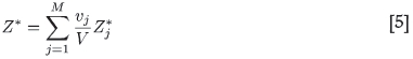
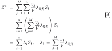
Assume that the total area(s) enclosed within the specified polygon(s) is denoted by V, and the supports of the M enclosed local estimates are referred to as 'blocks' vj. A kriged estimate Z*_j is available for each of these blocks. Then the 'global' kriged estimate that pertains to the entire area V is given by the weighted average (see for example, Journel and Huijbregts, 1978) of the Z*_j, i.e.

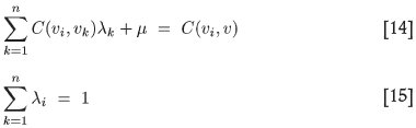
The proviso on this formula is that the same set of all η data samples be used to krige the Z*_j. Similar relations then hold for the 'global' weight λ_i pertaining to the contribution of the ith data sample to the estimate Z*, and also to the Lagrange multiplier µ in the event that ordinary kriging is employed:

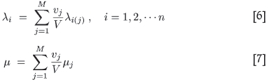
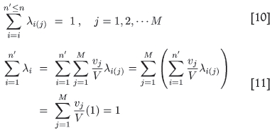
Recall again that Μ counts the number of blocks making up V and n the number of data points used to calculate the n weights λi(j₎, i = 1, 2,... n that give the kriged estimate of the jth block. From this, the above equation for the global weights follows,

A similar argument produces the 'global' Lagrange multiplier µ.

If it were simple to krige each block using all n available data values there would be no problem in producing the required global kriging variance associated with Z^*, since this error variance is given by

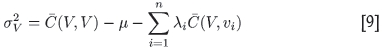
where the Lagrange multiplier µ < 0. In the case of SK, µ = 0. The global weights λ_i and the global Lagrange multiplier µ would be known from the above equations, and the covariances could be calculated straightforwardly from the variogram based on the smallest sample support. However, this is not the case.

As it stands, the implementation of the kriging equations to determine the λ_i(j) becomes impractical if the number of data points n is large (e.g. several hundreds or thousands, as would be the case here). Some of the weights become so small that rounding errors in the computer pose a serious problem.

 

The reduced data-set method (RDM)

An approximation to the above stringent requirements is clearly needed. One knows that only the 'nearest data neighbours' to the centre (or centre of gravity) of each block Vj are influential in determining Z*_j. Therefore an obvious approximation suggests itself: pretend that all the data values were used in kriging, but set artifically to zero the weights of those data samples that were not actually used to krige a specific block (and which are way out of variogram range anyway). Call this the 'reduced data method' or RDM for short. Although they used a different approach to calculating global kriging variances, Kim and Baafi (1984) alluded to this possibility, at least in theory. This dramatically reduces the number of data values required in kriging each block, and hence reduces the dimension of the corresponding matrix to be inverted.

This approximation yields results that are not too unreasonable for the global kriging variance in the case of SK, provided the number of data values n used per block is not too small.

For OK, the fact that the unbiasedness condition must be satisfied requires that the global weights sum to unity. This too is satisfied, provided the same requirement is met for the weights n^l< n, say, not set formally to zero:

As with most approximations, there is a price for introducing these simplifications: in artificially setting a selection of otherwise small but finite weights to zero, and implicitly leaving these data values out of the kriging equations, one finds that the global kriging variance is hugely overestimated.

Examples of the results obtained with this approximation for the test data are given next.

 

Results obtained with the RDM

For ease of reference, the first term in Equation [9] (the global kriging variance formula) will be called the polygon covariance term, the second term the global Lagrange multiplier, or µ, and the last term the sample/polygon term, sor sp.

Channel sample data was averaged into 239 60 m W 60 m blocks, and variograms based on the raw average gold accumulation values showed good structure (the histograms of block averages are only slightly skewed, allowing direct calculation on raw values, instead of on logarithms). For the purposes of this illustration, both the data and the unknown blocks to be estimated were taken to be of the same support, i.e. 60 m square blocks.

A rectangle of 18 W 5 (60 m) blocks, adjacent to the data blocks, was kriged (point kriging) using various schemes. Included in the latter was an exhaustive run for both OK and SK using all 239 blocks to krige every unknown block, with the idea that this would render the 'true' value for the global kriging variance in each case that one is striving for. This forms the last entry in the tables that follow. The other runs were based on using respectively n = 1, 2, 4, 8, 16, 32, 64 data samples to krige each block, for both OK and SK.

The polygon, for which the global kriging variance was estimated, included all 90 kriged blocks. The value obtained for the polygon covariance is, of course, a constant. The results obtained for SK are the following (global kriging variance in the last column):

 

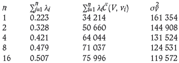
For values of n upwards of 16, a large number of negative weights are obtained and their impact is clear. Using a limited number of samples with which to krige each block does overestimate the global kriging variance, but not too dramatically.

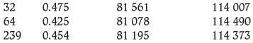
The results obtained for OK, under otherwise exactly the same circumstances, are the following:

The amount by which the global kriging variance is overestimated climbs drastically as the number of samples n used in OK is reduced.

Faced with the above problem, a study was made of how sp (the second column in the above tables) in the case of OK and SK, and -µ in the case of OK, decrease/increase with n, the number of samples used in kriging each block.

 

The link to the variancegram in the case of OK

The link to the variancegram will be illustrated graphically in the first place. The link will be made even though the variancegram is based on logvariance calculations, and the kriging was done on raw values. In fact, raw variances can be used as basis for the variancegram too, but in the case of Witwatersrand gold reefs the logvariances probably result in a more stable graph, which is very important.

We require the (log)variance as a function of the block side l. As was demonstrated (Figure 3), this function Γ(l) can be faithfully reproduced by a set of nested spherical variogram structures, as given in Equations [3] and [4].

An important requirement for the link is that the variancegram has to be fitted specifically up to a square side that is indicated by the total area defined by all the data blocks. In the case of the test exercise the total number of data blocks is 239 and they cover 239 W 3600 m², i.e. 860 400 m². The side of an equivalent square is 928 m. Thus the variancegram has to be refitted only up to 928 m, which changes the parameters somewhat.

The required fit to the variancegram was accomplished using five spherical variogram structures with parameters:

C₀ = 0

C1 = 0.710, a₁ = 20 m

C₂ = 0.280, a₂ = 60 m

C3 = 0.190, a₃ = 180 m

C₄ = 0.090, a₄ = 540 m

C₅ = 0.180, a₅ = 928 m

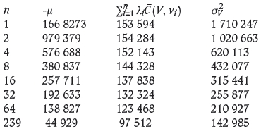
It is useful for the illustration to introduce the logvariance difference,

where the 'sill' in this equation can be any convenient value, since it will fall away in the final calculations.

We chose a sill of f(0) = 2.2276, the overall logvariance of the data area.

Inserting the above values for the fit of the variance-gram up to a square side l of 928 m, one obtains the graph in Figure 4 for ƒ(l) versus l.

 

 

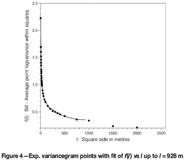
The global Lagrange parameter -µ in the case of OK

The remarkable finding is that the same behaviour as the above variancegram fit is displayed when -µ(n) is plotted against (n - 1), where n is the number of samples used in kriging. Figure 5 gives the experimental points obtained for the test data.

 

 

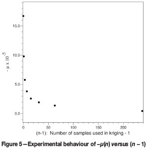
It is immediately clear from Figures 4 and 5 that these two graphs can be scaled to coincide, and the scaling constants will give proportionality criteria. Furthermore, when -µ is plotted versusƒ(l) (see Figure 11) the relationship is shown to be a linear one.

 

 

 

 

 

 

 

 

 

 

 

 

The variancegram is known beforehand, and therefore, three known points on the -µ versus (n - 1) curve will determine the scaling constants for the entire curve. This in turn enables one to determine -µ for a value of n of, say, 239 blocks, i.e. all the data blocks, which means that the correct value of the -µ component of the global kriging variance can be computed.

The actual determination of the scaling constants will be discussed below.

 

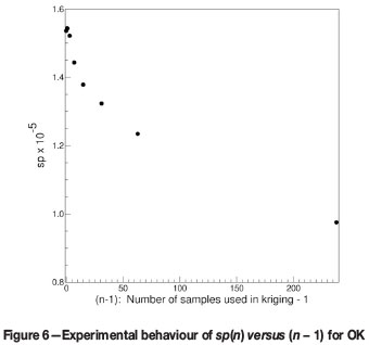
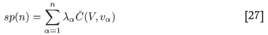
The sample/polygon term sp in the case of OK

sp(n) also decreases with (n-1), where n is the number of samples used in kriging. However, its behaviour is different from that of -µ(n) versus (n - 1), shown in Figure 5. Figure 6 gives the experimental points obtained for the test data when sp(n) is plotted versus (n - 1). There is not the immediate resemblance to the way in which ƒ(l) decreases with l.

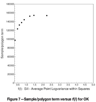
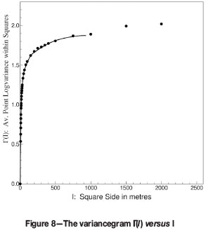
The scaling behaviour of sp is clearly more complicated than was the case for -µ. When sp is plotted versus ƒ(l) the result is a curve resembling Г(l) versus l. Figure 7 gives the former curve, and Figure 8 shows the latter for comparison.

The two curves can again be scaled to coincide, identifying the necessary scaling constants and allowing extrapolation to n = 239 for the correct value of sp(n).

The procedures are discussed below.

 

The link to the variancegram in the case of SK

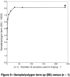
In the case of SK there is of course only the sample/polygon term to correct in the equation for the global kriging variance, since the Lagrange multiplier is absent. The procedure for correcting sp here is very similar to that used for correcting -µ in the case of OK, with only one difference: sp increases with n (see Figure 9) in a manner reminiscent of the way in which Γ(l) increases with l.

This means that the only change necessary in the approach used for -µ is a change in what ƒ(/) in Equation [12] now stands for:

By empirically scaling the axes in the respective graphs of sp versus (n - 1) and the newƒ(l) versus l, the two curves can again be made to coincide. The relationship is linear.

Note that for n = 64 and n = 239 in Figure 9, the large number of negative weights obtained have an impact on the experimental value of the sample/polygon term. The star in the graph indicates the calculated 'true' sp value for n = 239, which is unaffected by negative weights. Aside from that, it is not difficult to see that the above graph can be scaled to coincide withƒ(l) = Γ(l).

 

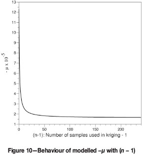
An approximate analytical model

In this section a simple analytical model kriging system is examined to obtain some insight into the behaviour of µ and sp for OK, for example, with increasing n. Analogous results can also be obtained for SK. The crux of the problem is to see if one can understand their behaviour from the structure and solutions of the kriging equations themselves. The OK kriging system to be solved is, as usual,

where n data points have been used to krige block v. To obtain approximate analytic solutions for the values of λ and µ for arbitrary n replace the off-diagonal elements C(v_i, v_k), for i ≠ k, by their common average, and the right hand terms C(v_i, v) by their average taken over all data points. Making the replacements

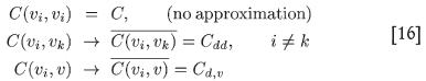
in Equation [14], the resulting system of equations can be solved exactly. One finds that λ_ί = 1/n for all i,

while µ is given by

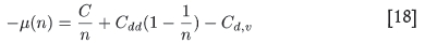
This exhibits the same qualitative behaviour as was seen empirically: for n = 1 the value is µ(1) = C - C_d,v, dropping down to a lower limit of µ(^∞) = C_dd - Q_d,v. A graph of the solution for - µ(n) is shown in Figure 10 (compare to Figure 5).

In generating this illustrative figure, the typical estimates C = 1.245 W 10⁶, C_dd = 0.187 W 10⁶, and C_d,v = 0.019 W 10⁶ have been used.

In this connection it is therefore important to realize that the strong n-dependence of µ arises solely as a consequence of the restriction. This condition forces the common λ values to equal 1/n, and thus the µ in Equation [18] to become a function of 1/n.

Note that the order of magnitude of the model values of sp(n) and -µ(n) are not expected to reproduce the empirical values, due to the extremely crude assumptions made. However, the model faithfully reproduces the qualitative behaviour of the empirical observations to a striking degree.

The application of the findings to the computing of correct global kriging variances from the variables obtained by local kriging is set out next.

 

Correcting global kriging variances in the case of OK

The correction procedures referred to above will be illustrated using the same exercise that was used previously: the data-set consisted of average gold accumulation values for 239 60 m W 60 m blocks, and it was used to krige an adjacent rectangle of 18 W 5 (60 m) blocks. The relevant distance over which the variancegram had to be fitted was 928 m.

As before:

where an arbitrary 'sill' value of 2.2276 (in this case the overall logvariance of the data area) was chosen for convenience, and Γ(l) reproduced the variancegram by means of a model fitted with five nested spherical structures:

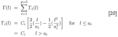
l denotes the side length of the square for which each logvariance is calculated in the experimental variancegram.

 

Methodology for correcting -µ, the global Lagrange parameter

It was found that -µ decreases with n, the number of samples used to krige each block, in a manner reminiscent of the way in which ƒ (l) decreases with l (see Figures 4 and 5). By empirically scaling the axes in the respective graphs, these two curves can be made to essentially coincide.

Mathematically this means that the variable pairs [-µ, ƒ (l] and [n, l] are linearly related. Hence we may write

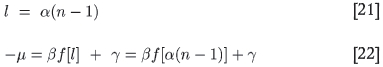
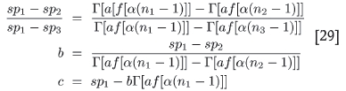
where the (n - 1) dependence on n is necessary since the minimum value of n is 1, and this has to be associated with the minimum value of l of the variancegram, which is zero. The function ƒ was defined in Equation [19]. The constants α, β, and γ perform the necessary scaling to cause the two curves in question to overlap. Since there are three of these unknowns, we need three sets of data input to determine them. From a practical viewpoint, one would expect to know values for small sample numbers n₁, n₂, n₃, say. Then, by manipulating Equation [22] one can solve in turn for α, β, and γ from

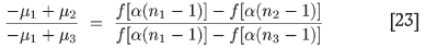
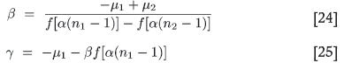
The notation is µ_i = µ(n_i). The first of these three relations is an equation for α. Once this has been solved, β and γ follow. To solve this equation we cross-multiply and set

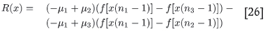
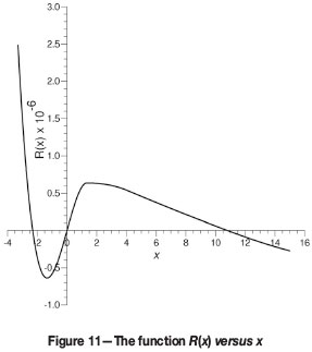
where x is a running variable. One sees that R(x) always passes through zero due to the form of f. Thus R(x) has one real root at x = 0; if R(x) were strictly a cubic polynomial in x one could argue for three real roots: one at 0, plus one negative and one positive root (we ignore the unphysical, but mathematically possible, outcome of one real root at zero, plus two complex conjugate roots). This is unfortunately not the case due to the discontinuities in the Г_i(l) that enter the form of f(l). However, if the real, positive root is not so large as to exceed the shortest range in Equation [20], one can perhaps expect R(x) to 'act' like a cubic. From the scaling hypothesis it is clear that α must always correspond to the positive, non-zero root. A specific example of how R(x) behaves when it has three real roots (the only case of practical interest) is shown in Figure 11.

A word of caution is in order here. If the coincidence of the -µ versus n and f versus l curves were exact, it would not matter which known values were used to obtain α, β and γ. However, since we are dealing with a so far empirically established relation which need not be exact, it will matter to some extent what input values are used. As it turns out, n₁ = 1, n₂ = 2, and n₃ = 8 or 16 or 32, etc. give very good results.

 

Methodology for correcting sp, the sample/polygon term

As was shown above, the sample/polygon term,, also exhibits a scaling behaviour, but one which is different from that of -µ. We first exploit the known l = α(n - 1) relation of Equation [21] to convert

to a function of =ƒ[a(n - 1)] instead of n. (This is what gave a straight line for -µ). In the case of sp, however, one finds a curve resembling Г(l) versus l (see Figures. 7 and 8). The two curves, sp versus ƒ and Γ versus l can again be scaled empirically to coincide. This means that

where a, b, c are three new scaling constants. The equations determining these have the same structure as Equations [23]-[25] with sp_i = sp(n_i) substituted for -µ_i and Γ[αf [α(n_i -l)]]for ƒ[α(n_i/-l)].Thus

 

The least squares fit modification

Instead of relying on the assumption that the straight line of -µ versus f in Equation [22] can be forced to pass through three of the data (experimental) points, which may lead to no real root for α in Equation [26], one can try a 'milder' approach of only requiring a fit in the least squares sense. This more robust procedure should always produce a solution, which is important for a production system. To do so one requires that the sum over the differences squared of S sample points that are going to be used to determine the scaling constants,

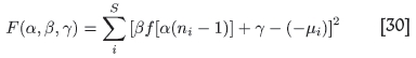
be minimized as a function of the parameters γ, β, and α. This means that

where f =f[a(ni - 1)] andf ^l is the derivative of(x) with respect to its argument x = α(n_i - 1). The first two equations are the usual least square conditions, arrived at by differentiating w.r.t. β and γ. The last equation is new. It arises upon differentiating w.r.t. α and requiring that this too should vanish. Then, upon defining

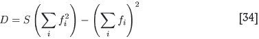
one finds, as usual, that

Substituting these two values into Equation [33], one finds an equation that determines the as-yet unknown α as a root of an algebraic equation, very much as in Equation [26].

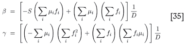
This equation can be recast as

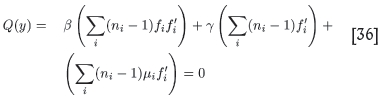
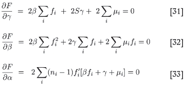
i.e. the value of y at which Q( y) vanishes is the preferred value of α. Once this has been determined, the preferred values of β and γ follow from Equation [35]. Next, one has to check that the solution so obtained indeed leads to a minimum value of F (α, β, γ), evaluated at these values of α, β, and γ. The condition for this to be the case is that all three second partial derivatives are positive there. Doing the calculations, one finds the three conditions

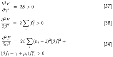
Of these, the first two are obviously always met: the third should be used as a test to ensure that one is indeed at a minimum of F as envisaged by the least squares problem. In the above development, pathological cases where Fis neither at a maximum or at a minimum have been excluded. One can check for such cases by verifying in addition that

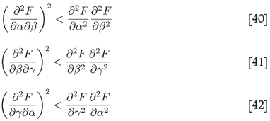
which, in combination with the vanishing first derivatives, guarantee a minimum or a maximum.

The derivatives of ƒ that are required come from Equation [19] with Equation [20] inserted for Г(l). Note that this consists of a sum of individual spherical variogram forms that have zero derivatives once the argument exceeds the range. This should be borne in mind in programming the derivative. One has

for the jth structure. Hence

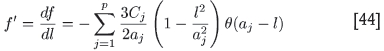
where the step function θ is merely a reminder that each term in the sum will contribute only provided l does not exceed its particular range a_j. The expressions for the required derivatives are

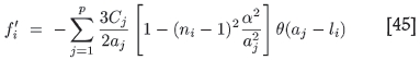
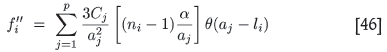
Notice that both derivatives are a sum over the p structures making up ƒ' and ƒ'', evaluated at the particular value l = l_i = (n_i - 1)α.

It is interesting to observe that in all cases where low values of n₁, n₂, n₃ were considered to obtain the scaling constants, the least squares method gave exactly the same values for the scaling constants as were found from the (largest) root of R(x) previously.

 

Calculation of a corrected -µ

To calculate the scaling constants for the test data the values for -µ(n_i) of [n₁, n₂, n₃] = [1, 2, 16] are used. Figure 11 shows the plot of R(x) versus x, the positive root of which will determine α .

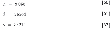
The value of the positive root in this case is x = 10.7968. This means that

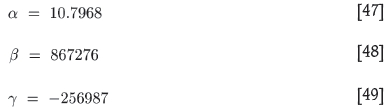
Knowing these constants, we can write the way -µ is expected to vary with the sample number (n - 1):

Extrapolating with this formula to n = 239, one finds

by direct calculation.

 

Verification of the scaling hypothesis for - µ

In order to verify that these scaling factors are indeed correct, we show the values of ƒ[10.7968(n - 1)], and the corresponding values of -µ(n) found in the kriging run:

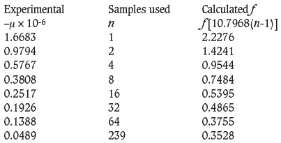
The number pairs [f, -µ] are plotted as closed circles in Figure 12.

 

 

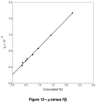
The straight line is given by Equation [22], plotted as a function of the variable ƒ. The agreement is truly remarkable!

The predicted point at n = 239 has also been included to illustrate that increasing values of n 'pile-up' on each other along the straight line of -µ versus ƒ.

It is useful to point out again that the inclusion of a sill to define the logvariance difference ƒ(l) = Sill - Γ(l) is merely one of convenience. From the previous development it is clear that one could equally well have considered -µ as a function of the variancegram Γ(l) = [α(n - 1)]. Then

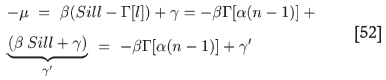
Here -µ is a linear function of the variancegram with gradient -β and a revised constant γ^l = Sill W β + γ. Thus the entire exercise of determining the scaling constants could equally well have been implemented by using the variancegram: the choice of a sill is irrelevant.

 

Calculation of a corrected sp

By cross-multiplying in Equation [29] one finds a function that is the exact analogue of R(x) in Equation [26]. The root of the former equation now gives the value of a in Equation [28] for fixed α. Using the input values of sp_i for [n₁, n₂, n₃] = [2, 4, 16] one determines the scaling constants as

Knowing these constants we can similarly write down an equation for sp versus n:

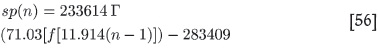
The extrapolation to n = 239 gives

Notice a small but important point: the value of α = 11.914 appears here instead of α = 10.7968. This happens because the samples for [n₁, n₂, n₃] = [2, 4, 16] were used for the sp, since sp₁ and sp₂ lie too close to give a useful determination of a, b, c. One must thus use the same n^ls for the coefficient α to remain consistent.

 

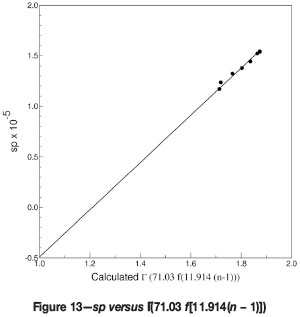
Verification of the scaling hypothesis for sp in the case of OK

We verify the linear behaviour again by evaluating Γ(n) = Γ(αƒ [α(n - 1)]) for the values at which the sp are known from the kriging runs

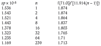
The straight line character of the plot sp versus Γ is verified in Figure 13.

 

 

Resulting estimated global kriging variance in the case of OK

The directly calculated ('true') OK global kriging variance for the test data is

The estimated OK global kriging variance based on the proposed correcting method is

As is clear from comparison of the above two equations, the estimated -µ and sp values are both higher than the true values, and since they are subtracted from each other, the resultant error in the global kriging variance should be reduced. However, the main source of discrepancy is the difference in the sp values. This could be ascribed to the fact that the true value of 97 512 is anomalously low due to the impact of negative weights, whereas the impact is absent in the estimated value.

Nevertheless, the estimated value exhibits an error of less than 11% of the true value, whereas the uncorrected RDM value based on kriging with 16 samples showed an error of 121%.

 

Correcting global kriging variances in the Case of SK

The correction procedure here focuses only on sp, since the Lagrange multiplier is absent. It was illustrated in Figure 9, that for SK, sp increases with n in a manner reminiscent of the way in which Γ(l) increases with l. This again means that the variable pairs [spƒ(l)] and [n, l] are linearly related.

Hence the rest of the formulism is exactly the same as was the case for -µ, except that -µ is everywhere replaced by sp, and ƒ(l) is reinterpreted as being Γ(l).

The least squares fit modification of the method to ensure a solution in a production environment follows immediately with the same replacements in the formulae of the relevant subsection above.

The experimental values obtained for sp in the case of SK based on kriging with n = 1, 2, 4, 8, etc. are given above. Using n₁ = 1, n₂ = 2 and n₃ = 16, the following scaling constants were obtained when solving the equivalent of Equations [23]-[25], replacing -µ by sp:

Knowing these constants, one can again write down the way sp is expected to vary with the sample number (n -1):

Extrapolating with this formula to n = 239, one finds

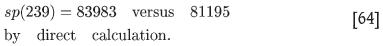
This estimated value for sp (239) is indicated by a star in Figure 9. It would indeed seem that this would have been the value of sp if the influence of negative weights were absent.

The scaling hypothesis for sp in the case of SK is verified next by evaluating ƒ(n) = Г[8.058(n - 1)] for the values at which the sp are known from the kriging runs.

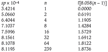
The straight line character of the plot sp versus Γ is again verified in Figure 14.

 

 

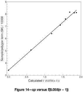
The deviations from the straight line at high n values are once more a manifestation of the impact of negative weights on the experimental sp values when kriging is actually performed with such large numbers of samples.

The directly calculated ('true') SK global kriging variance for the test data is

The estimated SK global kriging variance based on the proposed correcting method is

The estimated SK global kriging variance is within 2% of the true value, whereas the uncorrected RDM SK global kriging variance based on kriging with 16 samples is within 4.5% of the true value.

 

Conclusion

With research into new mining methods opening up the possibility of going to unprecedented depths in the Witwatersrand gold mines, the legacy of Krige's work remains as relevant as ever.

 

References

Journel, A.G., and Huijbregts, Ch. J. 1978, Mining Geostatistics. Academic Press, New York. 600 pp.         [ Links ]

Kim, Y.C., and Baafi, E.Y. 1984. Combining local kriging variances for short-term mine planning. Geostatistics for Natural Resources Characterization, Part 1. Verly, G., David, M., Journel, A.G., and Marechal, A. (eds.). D. Reidel, Dordrecht, The Netherlands. pp. 187.         [ Links ]

Krige, D.G. 1978. Lognormal-de Wijsian geostatistics for ore evaluation. Monograph Series M1. South African Institute of Mining and Metallurgy, Johannesburg. p. 26.         [ Links ]