Transferring sampling errors into geostatistical modelling

 

 

M. Cuba^I; O. Leuangthong^II; J. Ortiz^III

^IDepartment of Civil & Environmental Engineering, University of Alberta, Edmonton, Canada
^IISRK Consulting (Canada) Inc, Toronto, Canada
^IIIDepartment of Mining Engineering, University of Chile, Santiago, Chile

 

 

---

SYNOPSIS

Geostatistical modelling aims at providing unbiased estimates of the grades of elements of economic interest in mining operations, and assessing the associated uncertainty in these resources and reserves. Conventional practice consists of using the data as error-free values and performing the typical steps of data analysis -domaining, semivariogram analysis, and estimation/simulation. However, in many mature deposits, information comes from different drilling campaigns that were sometimes completed decades ago, when little or no quality assurance and quality control (QA/QC) procedures were available. Although this legacy data may have significant sampling errors, it provides valuable information and should be combined with more recent data that has been subject to strict QA/QC procedures.
In this paper we show that ignoring the errors associated with sample data considerably underestimates the uncertainty (and consequently the economic risk) associated with a mining project. We also provide a methodology to combine data with different sampling errors, thus preserving the relevant global and local statistics. The method consists of constructing consistent simulated sets of values at the sample locations, in order to reproduce the error of each drilling campaign and the spatial correlation of the grades. It is based on a Gibbs sampler, where at every sample location, the actual sample value (with error) is removed and a conditional distribution is calculated from simulated values at nearby sample locations. A value is drawn from that distribution and kept only if it satisfies some statistical requirements—specif-ically, the global relative error and local means and variances must be reproduced. All sample locations are visited and simulated sample values are generated iteratively, until the required statistics are satisfactorily attained over all sample locations. This generates one realization of possible sample values, respecting the fact that the actual samples are known to carry an error given by the global relative error. Multiple realizations of simulated sample values can be obtained by repeating the procedure. At the end of this procedure, at every sample location a set of simulated sample values is available that accounts for the imprecision of the information. Furthermore, within each realization, the simulated sample values are consistent with each other, reproducing the spatial continuity and local statistics. These simulated sets of sample values can then be used as input to conventional simulation on a full grid to assess the uncertainty in the final resources over large volumes. The methodology is presented and demonstrated using a synthetic data-set for clarity.

Keywords: sampling error, realizations of simulated sample values, uncertainty in final resources.

---

 

 

Introduction

In mineral resources/reserves modelling, the main and sometimes only source of information is the exploratory drilling data-set. During different stages of the project evaluation, various drilling campaigns are carried out in different periods of time and/or with different goals. As such, the exploratory data-set is continually updated by each campaign. The lifetime of an exploration project can be several decades, and in this context different technologies may be used during these drilling campaigns. Legacy data from campaigns drilled at early stages of the project may not have been subjected to any quality assurance and quality control (QA/QC) procedures¹ Even recent campaigns drilled will have different precision due to the drilling technique used, for example, diamond or reverse circulation drilling, or due to different QA/QC standards.

The effect of poor-quality data at different stages of a project has been widely discussed in the literature^2-4. The quantification of sampling error during sample collection and preparation for chemical analysis is also well documented; most operations perform routine checks of the quality of their sampling procedures^5-8.

One outstanding problem in the evaluation of mineral resources and reserves is the use of data with inherent errors. The use of imprecise data has been studied in the literature^4,9-11, but it is uncommon to find that the errors have been accounted for in the evaluation of the mineral inventory^12,13.

Regardless of the type of sample obtained during drilling campaigns, this data is the starting point for evaluating the quantity and quality of the various elements of interest. The quality of the final resource evaluation and the uncertainty quantification performed for risk assessment depend strongly on the data quality. Accounting for data quality from different campaigns has been addressed through very simple approximations such as adding an independent random error to each sample value³.

The present article deals with a methodology to incorporate sampling errors from different drilling campaigns into the geostatistical modelling process. The aim is to propagate the uncertainty associated with the data quality to all subsequent steps of the project evaluation, including risk related to the mine plan, classification of resources and reserves, transfer of geological risk into the financial performance of a project, and so forth.

We first review some fundamentals of sampling theory and of the geostatistical approach This is followed by an overview of the methodology and some details related to the simulation of multiple sample data-sets, in order to account for their precision. We provide some implementation details; and finally, we show an application to a synthetic data-set. We conclude with a discussion, recommendations, and future work.

 

Sampling error

When dealing with particulate materials, sampling theory provides a set of rules to ensure that some basic principles are followed when extracting a subset of the original volume in a representative manner. The original volume of material that is being characterized through the sampling process is called a lot^5,7. A sample is a small quantity of material extracted from the lot in such a manner that the sample represents the essential characteristics of the lot. Sampling as a process, however, aims at ensuring that the integrity of the sample is preserved.

The sampling process involves a stepwise reduction of the mass and the fragment size from the lot to the sample. The number of steps involved is a function of material characteristics and the requirements of the analytical procedure.

Diversions from this goal may be due to the characteristics of the material, the equipment used for increment extraction, the handling of increments after collection, and finally the analytical process itself.

In the case of samples from drilling campaigns, the lot corresponds to the drilled core of a given length or the detritus obtained in reverse circulation drilling, representing the extracted cylinder. From these lots, and after a series of stages of division of the total mass and reduction of the particles size through crushing and pulverizing, a sample, usually of a few grams, is obtained.

The goal of sampling is to obtain a selected sample that represents correctly some properties of the lot. Particularly, we are interested in the concentration (grade) of some elements that have economic interest. Inevitably, when selecting a subset of the lot, the sample will have properties slightly different from those of the lot. If sampling rules are strictly followed, there will be no bias, but some fluctuation or error around the true value should be expected.

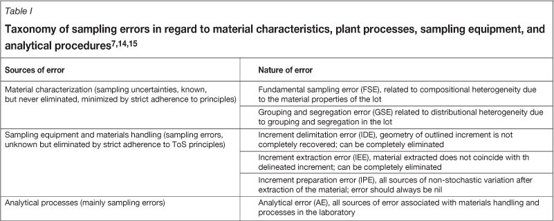
The theory of sampling (ToS) has developed a systematic taxonomy of errors and principles for minimizing or eliminating sampling errors. The combination of errors from these sources identified by Gy^5,.7,14 is termed the total sampling error (TSE). The relevant individual errors for this paper are shown in Table I.

Regardless of their type, the errors generate a difference between the sample properties and those of the lot. As long as each particle of the lot has an equal probability of belonging to the sample, there should be no bias; that is, in expected value the sample will have the same properties as the lot. However, some dispersion around the true value should be expected. A relative error quantifies this dispersion.

When accounting for all the sample locations, a global relative error (GRE) can be quantified:

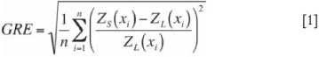
where n is the total number of sample locations, Z_s (x_i) is the sample value at location x_i, and Z_L (x_i) is the true value of the lot sampled at location x_i.

Sampling theory allows us to quantify some of the components of this global relative error, particularly, the fundamental sampling error (FSE). Other components cannot be directly quantified, but can be minimized through best practices, as they are related to the FSE and to the homogeneity of the lot, the number of increments to be used to compose the sample, proper sampling equipment design, etc.

 

Geostatistical approach

In geostatistical applications, a probabilistic approach based on the concept of random variables is used to account for our lack of information at unsampled locations. Similarly, we can consider that at those locations where we have a sample, but whose values are uncertain, random variables can represent these uncertainties. Specifically, we can assign a probability distribution to the attribute of interest, which in our context is the mineral or metal grade. It should be emphasized that locally the relative error should be of equal magnitude as the global relative error, but since the grade changes from one location to another, the dispersion is proportional to the grade value. This is, of course, a model of the spread of error around the true value. Other approaches could be considered⁴.

The distribution of the samples from a lot is frequently assumed to be Gaussian. However, experimental results have shown that this is not always the case, especially when dealing with precious metals with high nugget effect and highly skewed distributions⁷

From a geostatistical point of view, the lack of precision in the sample data can be accounted for by performing estimation or simulation conditional to data values that are independently drawn from the distribution at each sample location. This approach has been used before3. However, when significant relative errors are considered, one should also ensure that the spatial correlation between these simulated values at sample locations is preserved. If the values are simulated independently at every location, the spatial correlation will be partially lost and this will be reflected in the estimated or simulated models at subsequent stages. In the following section, we propose a methodology to handle data with different errors, imposing their spatial correlation and accounting for their precision.

 

Dealing with the sampling error

As mentioned, the common approach to accounting for sampling errors is to draw at each sample location a value from a distribution, usually Gaussian, centred at the sample value and with a variance proportional to the relative error associated. Since this process is done independently at each sample location, some spatial correlation is lost, and the simulated sample values show a higher nugget effect than the original values (with error), and the underlying actual values, which are unknown. This increase may not be relevant when the sampling error is low. However, when dealing with large relative errors, it may hide the actual continuity of the variable. This is illustrated in Figure 1.

 

 

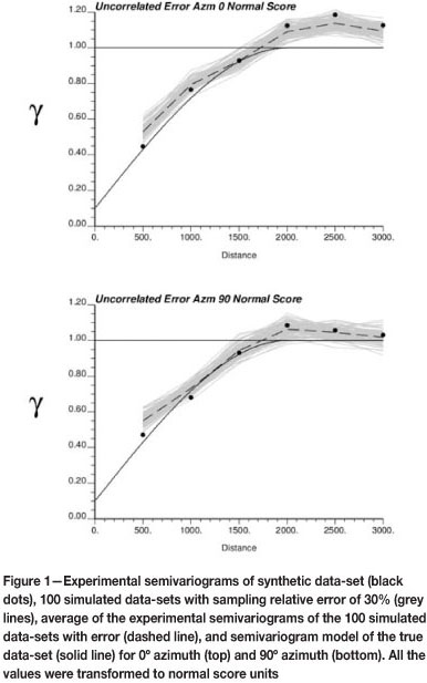
One other consequence of adding an independent sample error to the data values is an explicit addition to the variance of the data. As the sill of the variogram should be the variance of the data, this approach to explicitly account for sample error results in an inflation of the data variance and consequently, an increase in the variogram above the intended sill. Note further that while the variogram clearly rises above the sill, this should not be misinterpreted as a trend in the data. A trend demonstrated via the experimental variogram tends to show a consistently increasing slope beyond the range of correlation¹⁶. As such, the rise in the apparent sill above the standard sill is believed to be due to the sample error.

In conventional practice, the exploratory data-set of the mineral deposit is assumed to be error-free, and the experimental semivariogram of the data-set with its sampling error (from now on referred to as the available data-set) is used directly both for estimation and simulation. Since these techniques reproduce exactly the conditioning data, the conditional variance at such locations is zero, reflecting a misleading certainty about these values and underestimating the propagated uncertainty due to the actual imprecision at sample locations. This practice leads to an understatement of the actual uncertainty related to the resources of the deposit.

Based only on the available data-set and its respective sampling error (i.e. GRE), inference of the actual mean and variance is difficult; means and variances of the possible data-sets with sampling error could be smaller than, similar to, or larger than that of the data-set with no sampling error. Since we do not know the actual values without error, we must centre our statistical inference on the available data-set, which includes errors.

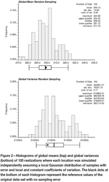
This can be illustrated with a simple example (see Figure 2). Let us assume the original data-set with no sampling error is accessible, and 100 realizations are sampled, assuming the distribution of samples with error for each data location is Gaussian, with a constant coefficient of variation in order to mimic a sampling process with error. Notice that means and variances of the simulated data-sets with sampling error can be smaller, similar or larger than those of the original data-set. Once we have a data-set with sampling error, we cannot infer if its statistical parameters are different than those of the error-free distribution, as this is dictated purely by chance. Since the error is added independently at every location, on average the distribution will show a higher global variance, as depicted in Figure 2 (right). This requires assuming the spatial correlation inferred from the data is not significantly affected by the sampling error, as we do not have access to the true underlying variogram.

 

 

The proposed approach considers simulating at the sampling locations, honouring the sample values in expected terms, and reproducing globally the GRE. Furthermore, the simulated values must retain the spatial correlation inferred from the available information. Notice that these constraints do not require the distribution at sample locations to be Gaussian-shaped. Each realization will represent a plausible set of samples obtained at the sample locations with the known precision provided by the GRE.

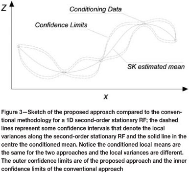
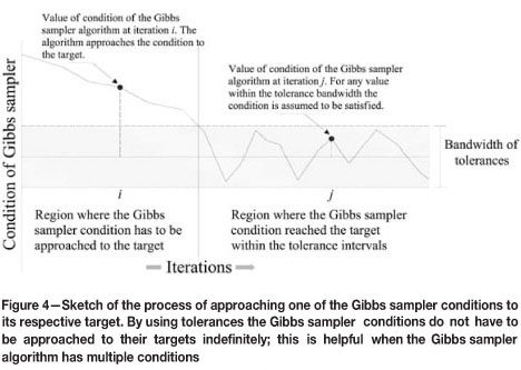
The Gibbs Sampler^17,18 works by selecting realizations from a second-order stationary random function, so that at the conditioning data locations they reproduce the GRE with respect to the available data-set; the variability due to the sampling error is transferred to the simulated model in terms of local means and variances (Figure 3).

 

 

Gibbs sampler algorithm for simulating additional data-sets

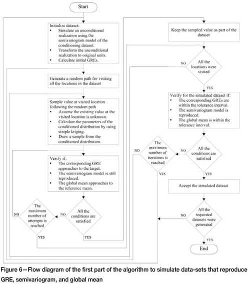
Since the experimental semivariogram has to be reproduced, a Gibbs sampling algorithm is used to generate the alternative data-sets, imposing the reproduction of the spatial structure and of global and local statistics. The sampling strategy splits the algorithm in two parts to speed up the processing time; however, this strategy is not rigid and many other alternatives based on the Gibbs sampler algorithm could be proposed to obtain the same results described here. Basically the aims of each part are as follows:

Reproduce the global mean, experimental semivar-iogram in normal score units, and the GRE values in the simulated subsets of values at sample locations; all of them within given tolerances. Each subset represents a drilling campaign and can have different GRE values
From the selected data-sets in the first part, adjust locally the local means to match the sample values; the reproduction of the experimental semivariogram in normal score units, and the GRE values are still preserved
For the Gibbs sampler algorithm, the back-transformations are carried out using the transformation table of the declustered available data-set. The sampling process is performed in Gaussian units since the conditioned distributions are parametric and the parameters can be easily and correctly calculated using the simple kriging (SK) approach. The experimental semivariograms are calculated from the normal score transformed values, since it is this semivariogram that is reproduced in simulation
The respective targets of the two parts of the Gibbs sampler algorithm are approached within some tolerance intervals. The use of tolerances helps to reduce the calculation time; they act as bandwidths of acceptable solutions with respect to the target values (see Figure 4). Conditions that have reached their respective targets within the tolerances do not continue trying to approach the target but move freely within the tolerance limits. This allows the algorithm to concentrate on the conditions that have yet to be met and not be stressed by conditions that are already acceptable, thus expediting the entire process
For the first part of the algorithm, a semivariogram model is fitted to the experimental semivariogram values of the available data-set in normal score units. Using this semivariogram model, several data-sets are simulated unconditionally to initialize the algorithm. Since the domain of the samples is finite, a smaller variance is obtained on average in the simulated datasets, since it represents the dispersion variance over the domain, rather than the theoretical variance. Since this bias affects equally high and low values in Gaussian units after back-transformation to original units, this may carry a bias in the global mean, depending on the skewness of the distribution. This bias is illustrated in Figure 5. When the starting realization has a significantly lower variance than the target, convergence to target statistics is hard to obtain. Therefore, for optimization purposes these realizations are discarded after a maximum number of iterations is performed without satisfactorily converging to the target statistics within their allowable tolerances.

 

 

 

 

The result of the first part of the algorithm (see Figure 6) is a set of simulated data-sets that honour the experimental semivariogram of the available data-set in normal score units, the GRE values for all the subgroups in the available data-set (each representing a drilling campaign), and the global means. Basically, this part of the algorithm filters out those unconditional realizations that are hard to solve, and delivers data-sets that are easy to solve for local correction to the second part of the algorithm. The workflow of the first part of the algorithm is summarized as follows:

1. Initialize the algorithm simulating an unconditional realization using the semivariogram model of the available data-set. The unconditional realization is simulated at sample locations. Back-transform the simulated values and calculate the respective GRE values for each subset, each representing a drilling campaign with different sampling error
2. Visit all the sample locations following a random path. The term iteration is used for one round when all the sample locations have been visited

a. Temporarily remove the value of the visited location and calculate the parameters of the conditioned distribution by simple kriging of the normal scores using the nearby values at sample locations. These are the values simulated unconditionally in the previous step
b. Draw a simulated value from the conditioned distribution
c. With the sampled value both in normal score and in original units respectively check if:

The GRE value of each subset approaches its respective target
The normal scores experimental semivariogram of the simulated data-set approaches the reference semivar-iogram. This is checked for several lags and directions
The global mean of the simulated data-set approaches the reference mean, in original units.

d. The term attempt is used for each time a sample is drawn from the conditioned distribution. For implementation, a limit in the number of attempts is restricted to a maximum value. If the sampled value satisfies all the conditions of step 2c accept the sampled value, keep it as part of the simulated data-set; otherwise reject it and go to step 2b.

3. The number of allowable iterations is restricted to a maximum value. When this value is reached the algorithm discards the simulated data-set and restarts from step 1. If the maximum number of iterations has not been reached, go to step 2. This part of the algorithm stops when all required realizations are completed.

 

 

The second part of the algorithm (see Figure 7) takes the simulated values from the first part and corrects the reproduction of the local means so that they are be equal to the available data-set within some tolerance intervals. The experimental semivariogram and the GRE were imposed in the first part of the algorithm and now move freely within the tolerance limits. Correcting the local means generates the following effects:

The GRE reproduction is better for all subsets, as it gets closer to the target values with less dispersion
The global means and global variances match the targets more closely
The nugget effect of the experimental semivariograms of the simulated data-sets increases; however, this is controlled by the tolerance in the reproduction of the experimental semivariograms.

 

 

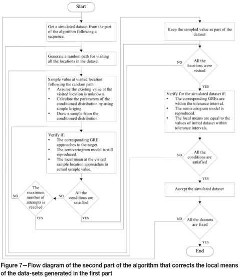
The summary of the second part of the algorithm is:

1. For each realization, take the simulated values from the first part of the algorithm
2. Visit all the locations following a random path

a. Temporarily remove the value of the visited location and calculate the parameters of the conditioned distribution by simple kriging of the normal scores of the nearby values at sample locations
b. Draw a simulated value from the conditioned distribution
c. With the sampled value both in normal score and in original scale units check if:

The GRE values approach to their respective targets
The experimental semivariogram of the simulated dataset approaches to the experimental semivariogram of the available data-set
Over all realizations, the mean of the simulated values at that particular sample location approaches the actual sample value (with error), which is assumed as the correct mean, since we do not have access to the error-free value.

d. For implementation, the number of attempts is restricted to a maximum value. If the sampled value satisfies all the conditions of step 2c accept the sampled value, keep it as part of the simulated data-set; otherwise reject it and go to step 2b.

3. The algorithm runs until the local means over the realizations at all sample locations are similar to the available data-set values within the given tolerances.

The resulting simulated data-sets now honour the GRE for all the subsets representing different drilling campaigns, the experimental semivariogram in normal score units, and the local means in original scale units.

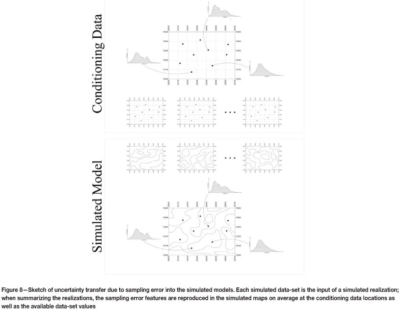
The data uncertainty due to sampling errors captured in the previous steps must now be transferred into the next step of geostatistical modelling. Each set of simulated data values is used as input in a three-dimensional conditional simulation model of the grades (see Figure 8).

 

Example implementation

To illustrate the practical implementation of this algorithm and how it would allow combining information from two different campaigns with different sampling errors, the following synthetic example has been prepared.

The goal is to account for these sampling errors in the subsequent step of simulation. The procedure is:

Generate 100 realizations of the values at sample locations, honouring the GRE, local values, and semivariogram in normal score units, using the proposed Gibbs sampler methodology
Simulate 100 realizations of the full grid conditioned on each case to one of the simulated sample data-sets
Compare the results with the uncertainty assessed when disregarding the sampling errors.

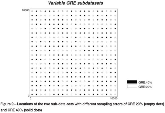
Let us consider an available data-set with 400 sample locations placed over a regular grid of 500x500 units of distance. The available data-set was split into two sub groups with a different sampling error associated with them. This was done in order to mimic the integration of two sampling campaigns in the study (see Figure 9). This available data-set was built sampling one realization over a regular grid and adding randomly a categorical code to each sample. The sampling errors were assigned according to categorical codes, GRE equal to 20% for code 1 and 40% for code 2.

 

 

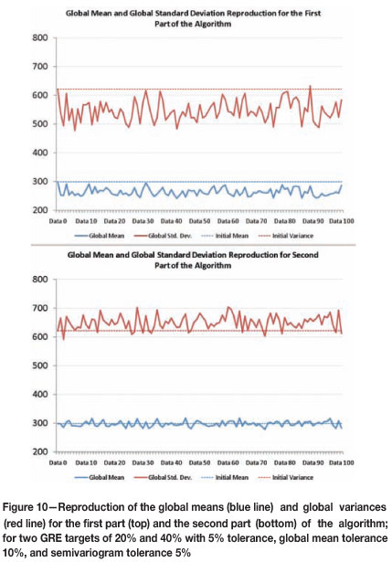
The Gibbs sampler algorithm runs in two parts. The first part tends to reduce the global means and global variances; however, this effect is corrected in the second part, where the dispersion is also reduced. Even when the global mean is fairly reproduced, the global variances are greater than the target of the available data-set (see Figure 10).

 

 

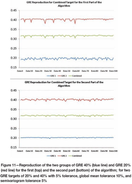
The variability in the reproduction of the GRE values for the two subsets is also reduced by the second part of the algorithm. In the first part, the GRE values are reproduced within the tolerance limits, and in the second part the dispersion is reduced (see Figure 11).

 

 

In the first part of the algorithm only the global conditions are targeted; the second part targets the reproduction of the local features. Although the first part of the algorithm starts with unconditional realizations, the GRE converges to the target values for each subset with subsequent iterations. This implies that the simulated values tend locally toward the measured sample values (with error), as shown in Figure 12 (top). When considering the average of the simulated values at a sample location, the second part of the algorithm allows a much better reproduction of the target values, that is, the values of the available data-set (Figure 12, bottom).

 

 

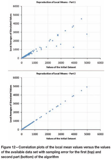
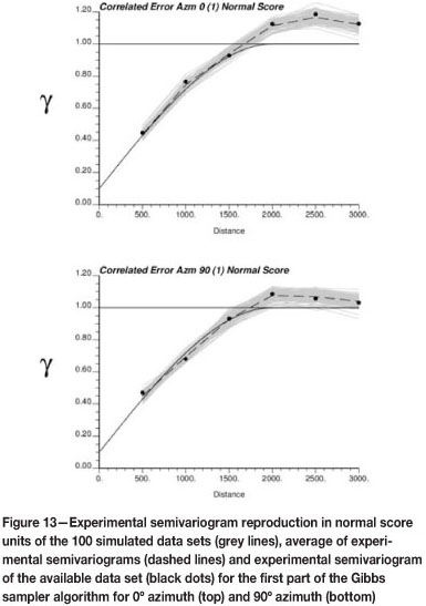
Figure 13 shows the reproduction of the semivariogram while accounting for the sampling error. Further, we note that the simulated data-sets also reproduce the semivariogram of the available data following the first part of the algorithm. It can be observed that the projection of the nugget effect is lower than in the case of adding an independent error to every location (Figure 1).

 

 

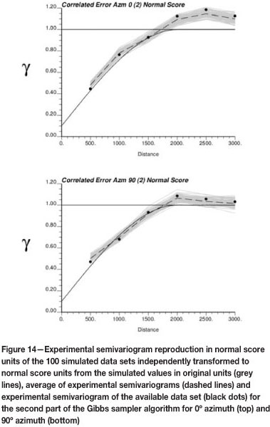
After the second part of the algorithm, the semivariogram reproduction improves and the dispersion between realizations is slightly lower (Figure 14).

 

 

Discussion

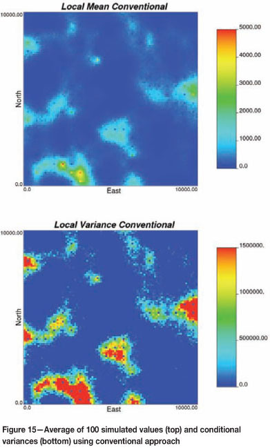
Recall that in the conventional approach, resource modelling depends on the available data-set, which is known to have errors. It is common to ignore the sample error and/or assume that an increased nugget effect in the semivariogram adequately accounts for sample errors in the final model. Conventional simulation modelling of resources then proceeds by (1) transforming the conditioning data (disregarding the sampling error) to normal score units, (2) fitting a semivariogram model, (3) simulating many realizations, (4) back-transforming to original units, and (5) summarizing the realizations in order to assess uncertainty (Figure 15 shows an example of one such summary).

 

 

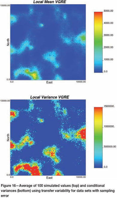
This paper proposes a methodology that accounts directly for sample error in the available data at the sample locations. The result of this proposed approach is a set of realizations of sample data at the sample locations. Each simulated data-set acts as the conditioning sample data used to generate each simulated realization. Resource modelling in this context requires that for each simulated data-set, we (1) transform the data to normal score units, (2) simulate one realization, and (3) back-transform the realization to original units. Semivariogram modelling is performed only once, on the original data-set. The uncertainty from this approach can be assessed once all realizations are generated. Figure 16 shows a similar summary of local means and variances as those shown in Figure 15, but the results in Figure 16 are based on the modelling approach outlined here. Notice that the variability at the sample locations is no longer zero but in fact reflects the uncertainty related to sampling quality.

 

 

 

 

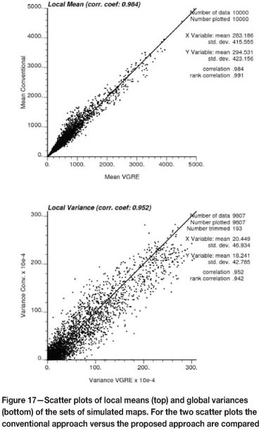
The average value at a sample location, over the set of realizations generated with the Gibbs Sampler algorithm, should be equal to the sample value (with error), since this is the only hard data available. However, since some tolerances were used in the second part of the algorithm, some fluctuations occur, as illustrated in Figure 17 (left). Globally, the allowable departure can be controlled at the expense of computation time for convergence (if more strict tolerances are imposed). In the case of the local variances, these are indirectly imposed by the global sampling error, but without local control (Figure 17, right).

 

 

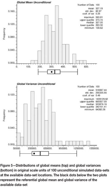
When comparing the distributions of the global means and variances of the conventional approach (see Figure 18) and of the proposed approach that reproduces the GRE at the sample locations (Figure 19), it can be seen that global means and global variances spread over a larger range in the proposed approach.

 

 

 

 

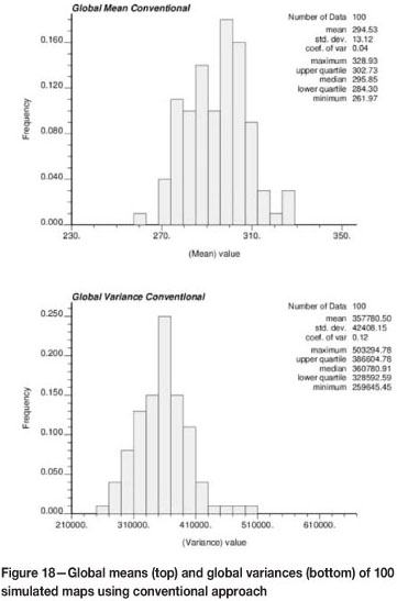
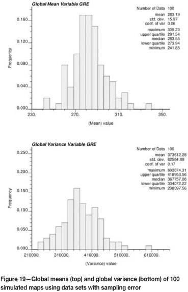
The global means for the proposed approach are centred on a value slightly lower than in the conventional case. However, global variances appear centred at a very similar value, with more dispersion in the case of the proposed approach. This can be explained by the fact that every realization is conditioned to a different set of samples and, therefore, the reference histogram changes. Depending on the distribution of high and low samples, accounting for the sampling error yet preserving the spatial correlation allows the global distribution to fluctuate. This is the result of transforming each simulated data-set independently and back-transforming the simulated maps using individual transformation tables.

 

Conclusions

Most widely used geostatistical techniques in the mining industry for building resource/reserve models assume that the conditioning information is error-free; conditioning data are perfectly reproduced at their respective locations in the geostatistical model. The uncertainty in the conditioning information cannot be accounted by using these techniques; therefore, it is not transferred into the geostatistical model. Since the exploratory data-set in mining consists of many different subsets corresponding to different drilling campaigns (e.g. reverse circulation drilling, diamond core drilling, or sampled information taken using technologies from different time periods or with different QA/QC standards), the presence of errors in the exploratory data-set is unavoidable. This should be accounted for in the characterization of the mineral deposit.

The present paper deals with errors in the data-set that arise from the sampling process, that is, the fundamental error. In practice there are additional sources of errors, such as errors in laboratory analysis or errors in manipulation of the sample, which cannot be easily quantified. A total error could be used with the proposed methodology, instead of only the fundamental error, as presented in the example.

The proposed approach is able to deal with many different subsets of information that comprise the exploratory data-set, each subset with a different sampling error. The general procedure consists of simulating alternative data-sets such that global statistics are preserved and the sampling error is imposed by considering that, at sample locations, the sample value is an outcome of a random variable with a mean given by the actually sampled value, which has an error, and a variance controlled by the amount of global relative error. These random variables are not independent, therefore the values are drawn using a Gibbs sampler in order to preserve the spatial correlation. Once the alternative data-sets have been simulated, each one feeds a simulated model constructed in the conventional way. The result is that overall uncertainty is increased when the sampling error is considered, demonstrating that assuming the samples to be error-free, when in fact they are not, leads to an understatement of the actual uncertainty in the resources and reserves.

 

Acknowledgments

The authors wish to acknowledge the three anonymous reviewers for their constructive comments that improved this paper.

 

References

1. WAKEFIELD, T. Legacy Data quality and its impact on mineral resource estimation. MININ 2008 - III International Conference on Mining Innovation. Arias, J., Castro, R., and Golosinski, T. (eds.). Gecamin Ltda. Santiago, Chile, 2008. pp. 3-10.         [ Links ]

2. VALLEE, M., AND SINCLAIR, A.J. Quality control of resource/reserve estimation—where do we go from here? CIM Bulletin, vol. 1022, 1998. pp. 55-57.         [ Links ]

3. MAGRI, E. AND ORTIZ, J. Estimation of economic losses due to poor blast hole sampling in open pits. Geostatistics 2000, Proceedings of the 6th international Geostatistics Congress, Cape Town, South Africa, 2000. Kleingeld, W.J. and Krige, D.G. (eds.), vol. 2, pp. 732-741, 10-14.         [ Links ]

4. EMERY, X., BERTINI, J.P., AND ORTIZ, J.M. Resource and reserve evaluation in the presence of imprecise data. CIM Bulletin, vol. 98, no 1089, 2005. pp. 2000        [ Links ]

5. Gy, P. Sampling of Particulate Materials—Theory and Practice. 2nd edn. Elsevier, Amsterdam, 1982. pp. 431.         [ Links ]

6. FRANÇOIS-BOMGARÇON, D. Geostatistical tools for the determination of fundamental sampling variances and minimum sample masses. Proceedings of the Fourth International Geostatistics Congress— Geostatistics Tróia'92. Soares, A. (ed.). Kluwer Academic, Dordrecht, 1993, vol. 2. pp. 989-1000.         [ Links ]

7. PITARD, F.F. Pierre Gy's Sampling Theory and Sampling Practice -Heterogeneity, Sampling Correctness and Statistical Process Control. 2nd edn. CRC Press, Boca Raton, Florida, 1993. pp. 488.         [ Links ]

8. MAGRI, E.J. Some experiences in heterogeneity tests and mine sampling. Proceedings of the Third World Conference on Sampling and Blending, Porto Alegre, Brazil, 23-25 October 2007. Costa, J.F.C.L. and Koppe, J.C. (eds.), Fundacao Luiz Englert, 2007. pp. 329-348.         [ Links ]

9. FREULON, X. Conditioning a Gaussian model with inequalities. Proceedings of the Fourth International Geostatistics Congress—Geostatistics Tróia'92. Soares, A. (ed.). Kluwer Academic, Dordrecht, 1993, vol. 1. pp. 201-212.         [ Links ]

10. FREULON, X. Conditional simulation of a Gaussian random vector with nonlinear and/or noisy observations. Geostatistical Simulations. Armstrong, M. and Dowd, P.A. (ed.). Kluwer Academic, Dordrecht, 1994. pp. 57-71.         [ Links ]

11. ZHU, H. AND JOURNEL, A.G. Formatting and integrating soft data: stochastic imaging via the Markov-Bayes algorithm. Proceedings of the Fourth International Geostatistics Congress—Geostatistics Tróia'92, Soares, A. (ed.). Kluwer Academic, Dordrecht, 1993, vol. 1. pp. 1-12.         [ Links ]

12. SINCLAIR, A.J. AND BLACKWELL, G.H. Applied Mineral Inventory Estimation. Cambridge University Press, Cambridge, 2002. pp. 381.         [ Links ]

13. ROLLEY, P.J. Geologic uncertainty in the development of an open pit mine: a risk analysis study. Unpublished M.Sc. thesis, University of Queensland, Australia, 2000. pp. 164.         [ Links ]

14. Gy, P. Sampling of discrete materials - a new introduction to the theory of sampling. I. Qualitative approach. Chemometrics and Intelligent Laboratory Systems, vol. 74, no. 1, 2004. pp. 7-24.         [ Links ]

15. Gy, P. Sampling of Heterogeneous and Dynamic Material Systems: Theories of Heterogeneity, Sampling and Homogenizing. Elsevier, Amsterdam, 1992. pp. 653.         [ Links ]

16. LEUANGTHONG, O. AND DEUTSCH, C.V. Transformation of residuals to avoid artifacts in geostatistical modelling with a trend. Mathematical Geology, vol. 36, no. 3, 2004. pp. 287-305.         [ Links ]

17. GEMAN, S. AND GEMAN, D. Stochastic relaxation, Gibbs distribution and the Bayesian restoration of images. IEEE Transactions on Pattern Analysis and Machine Intelligence, vol. 6, no. 6, 1984. pp. 721-741.         [ Links ]

18. EMERY, X. AND ORTIZ, J.M. Histogram and variogram inference in the multigaussian model. Stochastic Environmental Research and Risk Assessment, vol. 19, no. 1, 2005. pp. 48-58.         [ Links ]

 

 

© The Southern African Institute of Mining and Metallurgy, 2012.ISSN 2225-6253. Paper received Mar. 2009; revised paper received Oct. 2012.