TRANSACTION PAPERS

 

Novel size and shape measurements applied to jig plant performance analysis

 

 

A.E. Voigt^I; C. Twala^II

^IDebTech, De Beers Group Services (Pty) Ltd.
^IIKumba Iron Ore Ltd.

 

 

---

SYNOPSIS

Iron ore samples representing the input and output of several jigging experiments were analysed to determine the effect of particle size, shape, and density on jigging performance. Traditionally, the manual measurement of the size and shape of individual particles is very tedious and prone to inaccuracies and inconsistencies. Using a novel multi-view imaging technique the 3-dimensional representations of each particle in the sample was determined. From this representation several size and shape measurements were extracted, and these were correlated with the individual particle density measurements. A rigorous investigation into the confidence associated with density and the size and shape features as a function of sample size was conducted, thus allowing the significance of correlations in the data to be determined. The jig's performance was seen to be clearly sensitive to density and markedly so to particle size, while the results for shape indicated the need for continued work in the definition of particle shape.

Keywords: jig, MDS, size, shape, density.

---

 

 

Introduction

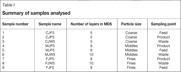
The Sishen Expansion Project (SEP) plant was designed to beneficiate low-grade ore (<60%Fe) in order to produce 13 Mt/a of product using jigging technology. Jigging technology was selected due to high cut densities of 4.2 g/cm³, required for low-grade ore beneficiation, as compared to those cut densities achievable in a dense medium plant. The SEP plant consists of five major sections: crushing, material preparation, beneficiation, final product handling, and quality control services. The beneficiation section is further divided into eight modules, which treat material classified into three size classes: the coarse fraction (-25 mm+8 mm), the medium fraction (-8 mm+3 mm) and the fine fraction (-3 mm+1 mm).

The quality control services utilizes the Mineral Density Separator (MDS) to predict and evaluate the performance of jigs. The MDS was developed by Mintek as a characterization tool to determine, in a jig simulating process, the response of an ore as a function of size, density, and shape of particles. It is used to fractionate samples into different density layers in which size and shape also play a role. The unit can treat material that falls within the size range 1 mm to 30 mm, with a step-up ratio of <4:1, depending on the particle density range of the material as well as the amount of near-density material. The technique employs similar separation principles to a jig, and utilizes only water and mechanical energy to lift the particles upwards, giving them a chance to settle onto a bed¹

Quantifying the effects of particle size and shape on a jig's performance has previously been difficult, as acquiring accurate individual 3-dimensional particle size and shape measurements on a large dataset is very time-consuming^2,3. This has meant that the resulting datasets are often too small to draw meaningful conclusions given the intra-class variation of these measurements, except in cases where the inter-class variation is large. In addition, because of this difficulty, shape factors are rarely measured on-line.

Recent developments in computer vision technology have enabled the accurate and rapid 3-dimensional (3D) analysis of particles⁴. Now, full individual 3D size, shape, and surface features can be measured at rates of tens per second, instead of one per minute. Correlating this with individual particle density has meant that the density measurement has now become the bottleneck in the data capturing process.

Quantifying the effects of particle size, shape, and density on the efficiency of a jig will assist in specifying the optimal input size, shape, and density ranges for a jig. Understanding the amount of variation in a particle parameter in a sample also allows the sample size to be optimally chosen, saving valuable laboratory time for on-site analysis.

 

Material description

Several samples were obtained from the coarse, medium, and fine jigs. These samples were made up of the feed, product, and waste samples, which were obtained using the ISO accredited automatic samplers. The feed, product, and waste samples were then further treated through the MDS. The output from each sample is several layers of material, each layer containing material of similar density, with layer 1 (which is heavier) at the bottom and layer 10 (which is lighter) at the top.

The material contains nine iron ore samples, each made up of several distinct layers as created by the MDS. No layer was lighter than 1 kg or heavier than 11 kg. Any single sample contains only particles of one of the size classes (fines, middles or coarse as described in the following section). The samples are described in Table I.

 

 

Experimental procedure

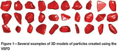
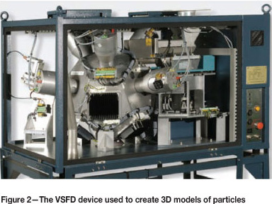
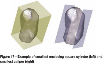
Each particle is individually imaged by a multi-camera imaging system called the VSFD (Vision Size Frequency Distribution) machine, shown in Figure 2. This device captures multiple simultaneous views of particles using six cameras at rates of up to 20 particles per second. Alternatively, batches of particles may be passed through the machine multiple times so that more views of each particle are created (in multiples of six). Using these views, an accurate 3D model of the particle is created as shown in Figure 1.

 

 

 

 

The particle's features are measured from this 3D model, and the accuracy of these features depends largely on the number of views available, the pixel resolution of the particle in the image, as well as the accuracy of the system's calibration⁵.

Two experiments were performed. In the first experiment, 1000 particles from each layer (72 000 particles in total) were measured by the VSFD and size and shape measurements were performed on the resulting 3D models of the particles. In the second experiment, density was correlated with the 3D models. As the density measurement was time-consuming, only the three samples from the coarse size range were analysed and the number of particles per layer was limited to 200 (3000 particles in total).

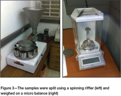
Care was taken to draw the particles (1000 or 200) from the layers in an unbiased manner. For this reason, a spinning riffler (Figure 3) was used to split the sample until the correct number of particles was obtained. A spinning riffler has been shown to be less influenced by operator bias than other sampling methods⁶.

 

 

Results

Jig sensitivity to particle features

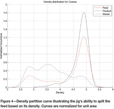
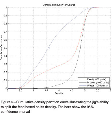
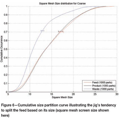
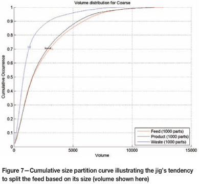
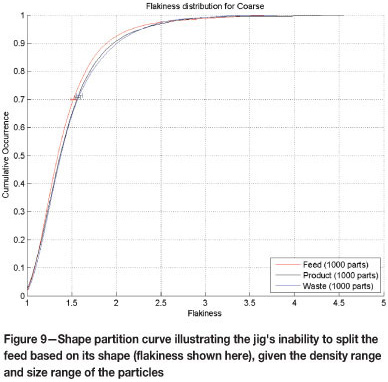
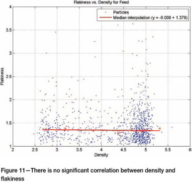
When data from all the layers in a sample is combined, the resulting distribution of a particle feature illustrates the sensitivity of the jig to this feature. The density, size, and shape sensitivity is illustrated in Figures 4-11 (for brevity, only volume, flakiness, compactness, and square mesh size are shown).

 

 

 

 

 

 

 

 

 

 

 

 

 

 

 

 

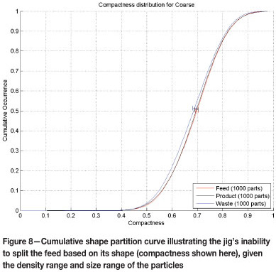
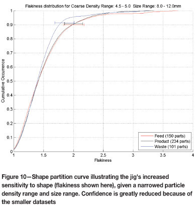
By constraining the plots to show only particles within a narrow density and size range, the sensitivity of the jig to shape is highlighted as shown in Figure 10. Note that by constraining the dataset, the number of particles per class is reduced and confidence is also reduced.

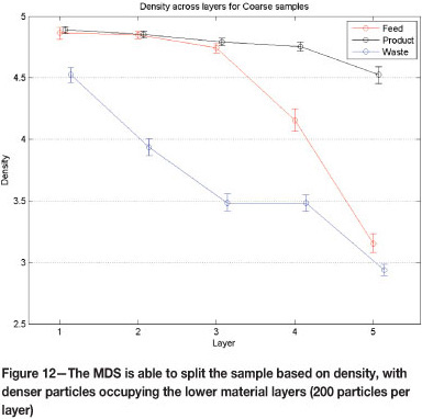
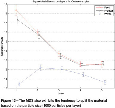
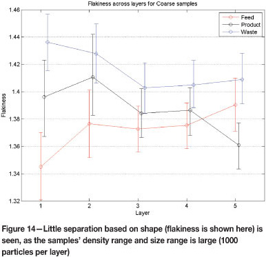
Analysis of MDS results

As the MDS device also uses a jigging action to separate particles, it is expected to exhibit similar sensitivities as a jig to the particle's properties. The MDS's separation performance is shown in Figures 12-14 (for brevity only the coarse sample's density, square mesh size and flakiness properties are plotted). The layer means and the 95% confidence interval of these means are plotted.

 

 

 

 

 

 

Undersized particles created by the sampling or handling of the material were removed by sieving the coarse, middles and fines samples with a 5 mm, 2.5 mm and 1 mm sieve respectively. Also, the VSFD machine's algorithms were set to ignore particles smaller than 2.5 mm, 1.5 mm, and 0.7 mm sieve respectively.

Particles were first weighed dry and then their submerged weight under water (at 20°C) was measured. These two measurements allow one to calculate the volume and density of the particle⁷ (Appendix A). Due to (a) the resolution setting used on the microbalance (1 mg), (b) fluid absorption by the particle and (c) in an effort to maintain a reasonable pace during density measurement, densities were measured to within 1% of the particle's actual density. In future, particles may be pre-soaked to eliminate the fluid absorption that some particles exhibited during submersion⁸. This might also better represent the actual conditions experienced on a jig. If fluid absorption took place (i.e. bubbles emanate from the particle after submersion), the particle's weight was taken 10 seconds after it was submerged.

 

Shape factors

The following size, shape^9, and density features were measured (these are defined in Appendix A):

  Flatness

  Elongation

  Compactness

  Convexity

  Surface roughness

  Volume

  Surface area

  Zingg shape class

  Sneed and Folk shape class

  Smallest enclosing square cylinder (emulates square mesh sieve)

  Smallest caliper (emulates gap sizing)

  Flakiness

  Weight from the microbalance

  Volume from the microbalance

  Density from the microbalance.

Shape classifications

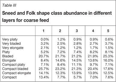
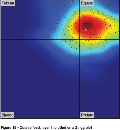
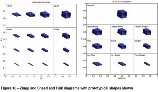
Particles were also classified using two standard shape classification schemes—Zingg plots and Sneed and Folk diagrams⁹ (see Appendix A). For brevity, only results for the Coarse sample (in experiment 1) are tabulated below, and only one Zingg plot is shown in Tables II and III.

 

 

 

 

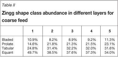
The classifications are shown in Figure 15. Each black datapoint represents a particle in the layer and the blue dot indicates the mean value of the dataset. The regions on the plot partitioned by the black lines are the shape classes as defined by Zingg. The shaded background indicates the plotted data point density.

 

 

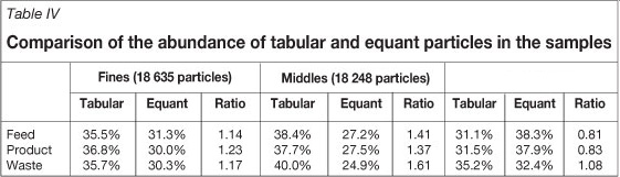
Calculating the ratio of the abundance of tabular to equant shape classes is a method to characterize the shape of the sample as a whole. This ratio was investigated for evidence of the jig's partitioning being affected by particle shape. Results are shown in Table IV, but show no consistent trend.

 

 

Concluding remarks

  The method described for rapidly determining density and 3D size and shape may be used in future to analyse the practical significance of various jigging parameters.

  The work shows that by ensuring samples are taken in an unbiased manner and by measuring individual particle densities accurately, a reasonably small sample size is required to construct density partition curves with high confidence. In future, this may allow more experimental cases to be considered when doing jigging experiments, as the measurement of density is now less tedious.

  For the samples analysed in this report, the jigging and MDS processes are seen to separate material mainly on density, although there is a clear tendency for particle size to influence the separation. The contribution from shape seems negligible and only a slight effect can be seen.

-  Even though a large number of shape features were measured, these do not necessarily capture the behaviour of the particle during the jigging process. A more appropriate shape measure is being investigated that takes into account the dynamics of the jigging process and the interactions that the particles experience in the process. These measurements are made on the existing 3D models.

-  When selecting (from the data) particles with a much narrower size and density distribution, it shows the sensitivity to shape more clearly. Unfortunately, by constraining the size and density range the sample size and confidence is reduced. Future work will include tailored particle sets with narrow size and density ranges and wide shape distributions to investigate the shape sensitivity of the process under constrained conditions while still having reasonably sized datasets.

-  From the shape abundance measurements (Table IV) on the given samples no clear indication that shape effects the performance of the jig is seen. Here again the contribution of shape is completely overwhelmed by the size and density sensitivity of the process.

  The 3D models correlated with density created in this study would be valuable as realistic particulate input into simulation studies being planned for iron ore processes

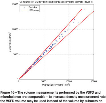
  Both the VSFD and micro balance estimate the volume of the particles. Both suffer from inaccuracies (e.g. the VSFD cannot see concavities and is limited by the number of views used; the microbalance loses resolution with small particles and is affected by the particle absorbing water). Figure 16 shows the volumes produced by both systems for one layer. For very small particles or large datasets, it would be more efficient to use the VSFD volumes and the microbalance weights to calculate density.

 

 

References

1. Green, R., Grobler, J., 2010. Vermaak, M., and Fouche, P. High density fractionation technique for lumpy iron ore. Symposium Series S61 Physical Beneficiation, Conference, CSIR, Pretoria, 4-6 May 2010, Johannesburg. The Southern African Institute of Mining and Metallurgy. pp. 115-125.         [ Links ]

2. Okonta, F. and Magagula, S. 2011. Railway Foundation properties of some South African quarry stones, Electronic Journal of Geotechnical Engineering, vol. 16 B. pp. 179-197.         [ Links ]

3. Wang, L., Lu, Y., Lane, D., and Druta, C. 2009. Portable image analysis system for characterization aggregate morphology. Transportation Research Record: Journal of the Transportation Research Board, vol. 2104. pp. 3-11.         [ Links ]

4. Forbes, K., Voigt, A., and Bodika, N. 2003. Using silhouette consistency constraints to build 3D models, Proceedings of the Fourteenth Annual Symposium of the Pattern Recognition Association of South Africa (PRASA 2003), Langebaan, South Africa, 27-28 November 2003.         [ Links ].

5. Forbes, K., Nicolls, F., De Jager, G., and Voigt, A. 2006. Shape-from-silhouette with two mirrors and an uncalibrated camera. Proceedings of the 9th European Conference on Computer Vision (ECCV 2006), Graz, Austria, 7-13 May 2006.         [ Links ]

6. Allen, T. Particle Size Measurement., Springer, vol. 1, 1996. pp. 4-7.         [ Links ]

7. ASTM. C693-93. Standard test method for density of glass by buoyancy. American Society for Testing and Materials, West Conshohocken, Pennsylvania, 1998.         [ Links ]

8. BSI. British Standard BS 2955. 1991. Glossary of Terms Relating to Particle Technology. British Standards Institution, London.         [ Links ]

9. Benn, D. and Ballantyne, C. 1993. The description and representation of particle shape. Earth Surface Processes and Landforms, vol. 18, pp. 665-672.         [ Links ]

 

 

Appendix A

Defining the particle characteristics (size, shape factors and density)

The following measurements are made using the 3D model of the particle as input:

  a, b, c—Caliper diameters along each of the particle's principal directions, resulting in three orthogonal measurements where 'a' is the longest caliper, 'b' the intermediate and 'c' the shortest. Measured in millimetres

  Flatness—A value larger than 1 related to the flatness of the particle and defined by the ratio of b:c. A sphere has flatness equal to 1

  Elongation—A value larger than 1 related to the elongation of the particle and defined by the ratio a:b. A sphere has elongation equal to 1

Compactness—A value smaller than 1 related to the compactness of the particle and defined by . A sphere's compactness measures 1

  Disk-rod—A value between 0 and 1 indicating where the particle lies along the disk (very flat like a square sheet of paper) to rod (very long and thin like a pencil) continuum. It is defined by the ratio (a-b):(a-c)

  Volume—The volume of the 3D model of the particle. Measured in cubic millimetres

  Smallest enclosing square cylinder—This measurement emulates the physical process of sieving using a square aperture sieve. Measured as the edge size of the smallest square hole the particle will pass straight through in millimetres

  Smallest caliper—This measurement emulates gap sizing. Measured as the smallest gap that the particle will pass straight through in millimetres (Figure 17)

 

 

  Flakiness—Calculated as the ratio of the smallest enclosing square cylinder to the smallest caliper

  Surface area—The surface area of the 3D model of the particle. Measured in square millimetres

  Convexity—A value between 0 and 1 indicating how convex the particle is and defined by the ratio volume:convex volume. The convex volume of a particle can be imagined as pulling a balloon tightly around a particle, thus covering any concave volumes around the particle. A coffee mug would for instance have its empty interior included in its convex volume where its volume itself excludes the empty interior. A sphere and cube have convexities of 1

  Surface roughness—A value bigger or equal to zero which measures the undulations on the particle's surface. It is defined as the sum of the higher spherical harmonic coefficients of the particle's surface. A sphere's surface roughness equals 0

  Zingg shape class—The particle's shape is classified into one of four classes as defined by Zingg⁹. These classifications are based on the a, b, and c measurements and are illustrated in the figure below:

  Sneed and Folk shape class—The particle's shape is classified into one of ten classes as defined by Sneed and Folk⁹. These classifications are based on the a, b, and c measurements and are illustrated in Figure 18. For the purposes of this report, Sneed and Folk diagrams are plotted as biaxial graphs and not as ternary diagrams as are done traditionally.

 

 

The following measurements are made using the microbalance:

  Dry weight—Measured in milligrams

  Submerged weight—The particle is weighed while submerged in water at 20°C

  Volume—The particle's submerged weight is equal to its dry weight minus the weight of the water that it displaces. Thus, the difference of the dry and submerged weight measurements divided by the density of water gives the volume of the particle measured in cubic millimetres

  Density—The dry weight divided by the volume of the particle gives the density of the particle in kilograms per litre.