TRANSACTION PAPERS

 

Assessment of the precision and bias of an online gauge using a single reference instrument

 

 

F. Lombard^I; G.J. Lyman^II

^IDepartment of Statistics, University of Johannesburg
^IIMaterials Sampling & Consulting, Pty. Ltd. Australia

 

 

---

SYNOPSIS

We consider the Grubbs estimation of the precision of an online gauge. Typically, this type of estimation involves independent results from two or more reference instruments (sampling and laboratory analysis operations). The properties of the estimator are then independent of the product variability. However, the use of more than one reference instrument entails significant additional costs.
The two-instrument Grubbs estimator, which is based on results from a gauge and a single reference instrument, has the disadvantage that its standard error is heavily dependent on the degree of product variability. We propose a new estimator that has a variance that is more or less independent of product variability. In fact, the variance is typically less than that of the Grubbs estimator based on the use of two reference instruments.
In order to function successfully, our methodology requires some prior knowledge of the extent of product variability and of gauge precision. In practice, such prior knowledge is often available and it is a weakness of the traditional two - and three-instrument Grubbs methods that no use is made of such knowledge. The efficacy and robustness of the new method is illustrated by Monte Carlo simulation.

Keywords: precision estimation, Grubbs estimator, Online analyser, ISO 15239, instrument variance.

---

 

 

Introduction

Consider measurement of a quality characteristic of a batch of product, e.g. coal, by each of two instruments. An application of particular interest occurs when one is considering the use of an online gauge as a substitute for a traditional but, in the long run, more costly and time-consuming sampling and laboratory analysis procedure. In order to judge the worth of a gauge, one would want to know its precision and also whether there is a bias between the results it reports and the corresponding results reported by a conventional sampling and analysis operation (the reference instrument). The standard method used to estimate gauge precision is the threeinstrument Grubbs¹ method. This method involves a comparison between results produced by the gauge and corresponding results produced by two independent reference instruments. The landmark paper by Rose² can fairly be said to have led to the establishment of the three-instrument Grubbs estimator as the estimator of choice in the coal industry for dealing with on-line analyser precision. Rose² gives examples of how the reference instruments may be arranged. Invariably, a second, independent sampling operation is required. Clearly, an additional sampling and analysis operation entails significantly increased costs for the duration of the trial. If stopped-belt sampling is involved, there will also be disruption of production.

Rose² discusses briefly the possibility of using a two-instrument Grubbs¹ estimation procedure, that is, where only one reference instrument, instead of two independent ones, is required. A problem with this method, also alluded to by Rose², is that the stability of the resulting estimate is adversely affected by large day-to-day variations in the coal quality. Such variations often leads to an estimate of gauge variance that is negative. The threeinstrument Grubbs estimator is not troubled by the effect of day-to-day variation, as this is eliminated by working with the pairwise differences between results rather than with the raw results. An obvious way to increase the stability of the two-instrument Grubbs estimator is to increase the duration of the trial, i.e. the number of samples that are taken. This, in general, is not cost effective. Calculations based on realistic scenarios indicate that hundreds of samples might be needed in order to obtain an acceptably precise estimate of gauge measurement error. The question arises, therefore, whether there is perhaps another way in which the stability of the two-instrument Grubbs estimator might be improved.

The purpose of the present paper is to show that such an improvement can indeed be effected under generally prevailing operating conditions. To understand why such improvement is possible, one should notice that in calculating Grubbs estimators no use whatsoever is made of any prior knowledge that may be available regarding the coal and gauge measurement variances. In other words, there is an implicit assumption that one knows nothing about the properties of the coal analysis technique and of the gauge measurements. In fact, statistical analysis of historical assay results can provide a good prior estimate of coal sampling and analysis variability and overall coal quality variability. Furthermore, the gauge manufacturer invariably supplies some guarantee regarding the precision of the gauge, which implies that there is reasonably accurate information available in that regard too. In any event, one can obtain a preliminary estimate of gauge variance from variographic analysis³ of the run of readings collected during the passage of a number of lots which are used to calibrate the gauge. Under normal circumstances, therefore, it will not be difficult to produce a reasonable prior estimate, w, of the ratio, w0, of true coal variance to true gauge measurement variance. We will show that the two-instrument Grubbs estimator of gauge variance can be improved substantially, at no extra cost, by the simple device of sorting the observed pairs of observations into a number of judiciously chosen subsets on the basis of the estimated ratio w. Two-instrument Grubbs estimators are then calculated within each of the subsets.

The effect of the sorting into subsets is that coal quality variation within any subset is smaller than the overall coal quality variation, hence the effect on the variance of the two-instrument Grubbs estimator is similarly smaller. When the estimators from each of the subsets are averaged, an estimator which has greatly reduced variance results. In fact, the new estimator typically performs substantially better than either of the Grubbs estimators. This finding has far-reaching implications regarding the costs involved in an operational comparison between an online gauge and a sampling and analysis procedure. A two-instrument Grubbs estimation using n laboratory results might be judged equivalent in cost to a three-instrument estimation involving n/2 results from each of two independent sampling and analysis operations. The actual cost of taking the additional set of n/2 samples will, however, be considerably greater because an automatic sampler, which is likely to be available for taking the first sample (instrument 2), is unlikely to be available for taking the sample corresponding to instrument 3. Manual acquisition of the instrument 3 samples will then be more costly than the instrument 2 samples, and may also be biased if cut manually from the stream of coal without using stopped-belt sampling.

The new method proposed here is not a panacea, however. It will be applicable only if reasonably accurate prior knowledge of the extent of coal quality variability and of gauge measurement variance is available. If the prior information regarding either or both of these uncertainties is far off the mark, the method could produce a grossly incorrect estimate of gauge error. However, as remarked above, it is seldom the case that reasonably accurate prior information is not available. Hence, it will generally be safe to implement the new method. The potential savings in respect of time and additional sampling and analysis costs certainly make the method worth considering as an alternative to the traditional three-instrument Grubbs estimator.

Later we give an overview of the Grubbs estimation methodology and provide examples of the numerical calculations involved. We give a formal definition of the new estimator. We also show how the standard error of the new estimator is calculated. We use Monte Carlo simulation to compare the variance of the new estimator to the variances of the original two-instrument and three-instrument Grubbs estimators. The results suggest that the new estimator can perform substantially better than either of the Grubbs estimators in terms of statistical efficiency. We also give an example of the calculations required to determine ahead of time the number of samples required to estimate gauge precision with a pre-specified standard error. Finally, we discuss how the data might be used to detect biases in the gauge calibration.

 

The Grubbs estimators

Table I shows a small subset of a larger set of data collected in a gauge evaluation. The rows, which correspond to successive days, are determinations of the specific energy of coal sampled from a moving stream by three instruments: an online gauge, a mechanical sampling and laboratory analysis procedure, and an independent manual sampling and laboratory analysis procedure. (This data is used purely for illustrative purposes and is not intended to reflect any particular reality).

 

 

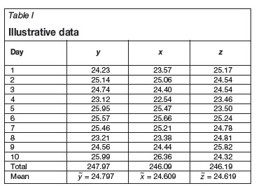
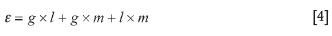
The three numbers (y x z) in any given row can be represented by the following three equations:

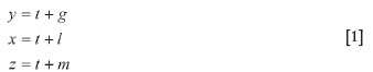
where t denotes the (unknown) 'true' specific energy value of the coal and g, l, and m denote the measurement errors associated with the three instruments. The measurement errors l and m associated with the two sampling and analysis procedures consist of the sum of the sampling, preparation, and analysis errors. For simplicity of presentation, we assume for the moment that no biases are present between the three instruments. Bias is dealt with later. The extents of the measurement errors are quantified by their respective variances, denoted here by , , and , the primary objective being to obtain a reliable estimate of . Notice that none of the four variables of interest, namely g,l,m, or t are observable. Thus, the challenge is to estimate using only the three observables y, x, and z. Towards this goal notice that

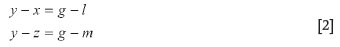
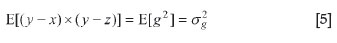
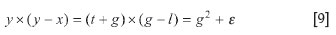
which eliminates t from consideration, and that

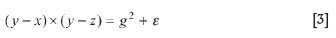
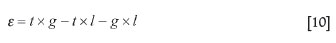
where

Under the very reasonable assumption that the measurement errors of the instruments are statistically uncorrelated it follows that the expected value E(ε) is zero, whence

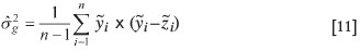
Here and elsewhere in the paper, the expected value of a quantity denotes its average value over the ensemble consisting of all its possible realizations. Consequently, it is sensible to estimate by the average of the n (= 10 in the particular instance of Table I) observed realizations of the quantity (y-x) × (y-z):

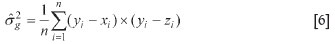
A small adjustment must be made to the last formula if the presence of constant offsets (biases) between the instruments is to be accommodated. Namely, each of yi,xi and zi must be reduced by the corresponding mean over all days (e.g. yi must be replaced by ỹi = yi - y ) and n must be replaced by n - 1, so that

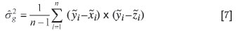
Notice that the variances and of the reference instruments can be estimated in exactly the same way by simply interchanging appropriately the roles of yi,xi, and zi in the last formula. The standard error of is given by Grubbs¹:

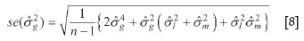
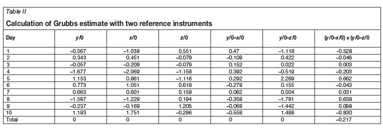
Table II sets out the calculation of for the data shown in Table I.

We find = -0.217/9 = -0.024, which is not a useful result and which in practice would be interpreted as saying that the gauge measures specific energy with no error. Using similar calculations, we find = 0.138 and = 1.645. One explanation for the negative gauge variance estimate is that the variances of the reference instruments are apparently one to two orders of magnitude larger than the gauge variance. If a reference instrument is of poor quality one can hardly expect to obtain a useful outcome when evaluating against it an instrument (such as a nuclear gauge) that has much better precision, unless the number of samples is increased from 10 to a substantially larger number. However, we will see later that the new estimator gives a sensible result from these 10 observations alone.

Rose² recommends that in general at least 60 samples of data should be gathered in order to obtain a useful estimate of . If stopped-belt sampling is involved, this recommendation implies a costly interruption of the normal production process for an extended period of time. Accordingly, Rose² considers also Grubbs estimation involving only y and x observations (no data from stopped-belt sampling). That an estimate of can also be made in this setup follows upon noticing that

where now

Assuming that the two measurement errors are statistically uncorrelated and also uncorrelated with the true value t, then E(ε) is again zero and an argument analogous to that used in the three-instrument case shows that can be estimated by

The standard error of in this context is given by Equation [8] with there replaced by

The calculation of using only the data in the y and x columns in Table I is set out in Table III.

 

 

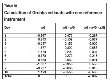
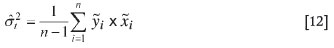
We find = -0.889/9 = -0.099, which is again not a useful result. The estimated standard error, calculated using the prescription given Table III is 0.121 (it is a moot point whether it makes sense to quote a standard error in respect of a negative variance estimate). The result is indicative of the statistical price to be paid for the benefit of eliminating a third instrument-many more samples are typically required if a useful estimate of gauge variance is to be made. Here the primary reason for the negative variance estimate is the large coal quality variance that the Grubbs method estimates as = 1.168 (see Equation [12]). This happens because in a two-instrument setup functions essentially as the variance of a fictitious third instrument against which the gauge is being compared. The estimation method described in the next section is a modification of the preceding two-instrument (gauge and one reference instrument) Grubbs method that ameliorates the effect of large coal quality variances.

 

The new estimator

In the interest of clarity we define our notation anew. A typical value, y, reported by the gauge can be represented as

where t denotes the true value of the quality characteristic in question as seen by the gauge and g denotes the statistical error intrinsic to gauge measurements. The latter error is assumed to have a distribution with zero mean and variance . Similarly, a typical value, x, produced by sampling and laboratory analysis can be represented as

where α + t denotes the true value as seen by the sampling and laboratory analysis and where l, the statistical error due to sampling and laboratory analysis, has a distribution with zero mean and variance . Equation [14] incorporates the possibility of a constant bias, α, between the results produced by the two instruments. Note that neither of these two equations tells us which of the instruments is, in fact, producing biased readings. The standard error of the new estimator will not be affected in any way by the presence of such a bias. The data for analysis is a set of n (assumed to be an even number) pairs of observations (y1, x1),..., (yn,xn) obtained from n batches of coal. The true values of the batches are not constant and are assumed to vary in a statistical manner around a mean µ, the average long-term analyte value as seen by the gauge, with a variance which quantifies the batch-to-batch variation.

Description of the estimation method

A general description of the method is given first, followed by a numerical example. With each pair of observations (y, x), associate a weighted average

where the weight w is an a priori estimate of the numerical value of the ratio

From (13) and (14) we see that the conditional expected value of d is

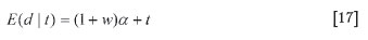
so that d serves as an indicator of the quality of the batch in question. We have n such d-values. Arrange these in increasing order of magnitude, d₁<L <d_n say, and form the m = n/2 subsets

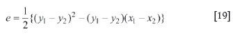
There are two observation pairs, denoted by (y1, x1) and (y2, x2), associated with each subset. For each subset we now calculate the corresponding two-instrument Grubbs estimator using only these two pairs of observations, namely

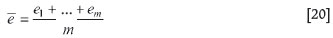
Doing this for each subset yields m estimates e1,..., em. The new estimate of is the average of these m estimates:

The sampling and analysis variance may be similarly estimated simply by interchanging the roles of y and x and replacing by in the preceding algorithm.

The motivation for sorting into subsets is that coal quality variation within any subset is typically substantially smaller than the overall quality variation, hence the effect on the variance of the two-instrument Grubbs estimator is similarly smaller. When the estimators from each of the subsets are averaged, an estimator which has greatly reduced variance results.

Numerical illustration

The calculation of the new estimator will now be illustrated using the small set of specific energy (MJ/kg) determinations shown in Table IV. Prior estimates of σt and σg are given as 1.15 and 0.23 respectively. (This data is used purely for illustrative purposes and is not intended to reflect any particular reality.) We used w = (1.15/0.23)2 = 25 in the calculation so that d = 26x -25y; see Equation [15].

 

 

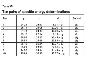
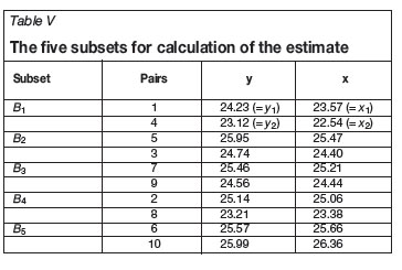
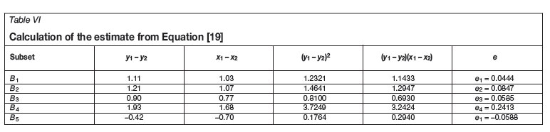
Table V shows the five subsets of observation pairs and Table VI shows the calculation of the ei value using Equation [19].

 

 

The mean of the five ei values is e = 0.0740, which is the estimate of the gauge variance . In this particular instance, we saw earlier that the standard two-instrument Grubbs estimate is = -0.099, which is uninformative.

Standard error of the estimator

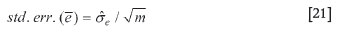
There is a simple formula for the standard error associated with the new estimator, namely

where

In the numerical example above, = 0.1082 and the standard error associated with the estimate = 0.0740 is 0.1082/ = 0.0484. In contrast, the standard error associated with the standard two-instrument Grubbs estimator of gauge variance is 0.121. This is about two and a half times larger than the standard error of the new estimate. We can also see from the fourth column in Table VII how the improvement by the new estimator comes about. The coal quality variance within a subset is estimated by (y1-y2)(x1-x2)/2. The estimates of quality variance within each of the five subsets are thus 0.571, 0.647, 0.347, 1.621, and 0.147, with an average of 0.667. This is a little more than half the overall estimated quality variance of 1.168 found earlier-see below Equation [12].

 

 

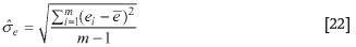
Equation [21] arises from the fact that the values e1, K, em are, to good approximation, statistically uncorrelated and have a common, albeit unknown, variance . The mathematical details of the argument leading to Equation [21] are available from the authors as a separate document. Suffice it to point out here that the structure of d in Equation [15] plays a crucial role in the analysis. The simulation results shown later can be used to verify the result empirically in three specific instances.

It will often be more convenient to estimate directly the standard deviation, σg, rather than the variance, of the gauge error. Then the estimate of σg is with standard error

Thus, in the numerical example above, the estimate of gauge error standard deviation is with an associated standard error of:

It is entirely possible, especially if σt is an order of magnitude or more larger than σg, that some values among the ei will be negative. When this occurs we simply eliminate from consideration the negative ei values. Thus, the new estimator is more properly defined as the average of the positive ei. However, in calculating σˆe we use all the ei, both positive and negative. This safeguards a user against gaining an over-optimistic impression of the precision of the estimator. Of course, if σt is excessively large, then any two instrument method will fail because the effect of σt cannot be eliminated entirely unless a third instrument is involved. In the remainder of the paper we assume without further mention that this modified version of the estimator is the one under discussion. In particular, then m denotes the number of positive ei values.

 

Efficiency of the estimator

The efficiency of the new estimator relative to the standard two- and three-instrument Grubbs estimators will now be illustrated by Monte Carlo experiments. The efficiency of the new estimator is defined as the ratio of the variance of (either of) the Grubbs estimators to that of the new estimator.

Monte Carlo simulations

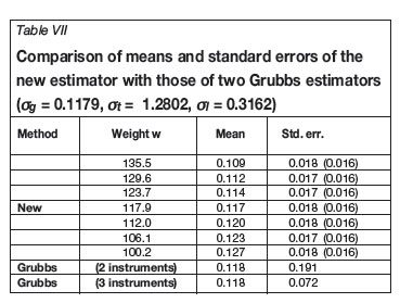
The following parameter configuration is motivated by data obtained in the evaluation of a PGNAA online coal analyser: σg = 0.1179, σl = 0.3162, σt = 1.2808, and n = 94. Thus, the value of w0 in Equation [16] is 117.85 (= 1.28022/0.11792) in this particular instance. We simulated the estimation procedure using seven different values of w in Equation [15], namely w = 135.5, 129.6, 123.7, 117.9, 112.0, 106.1, and 100.2.

The first three and last three of the latter values correspond to incorrect specification of the correct value wo by 5%, 10%, and 15% respectively. Using normally distributed random numbers, 1 000 samples were generated, each consisting of 94 pairs of observations following the given parameter configuration. The new estimate, , was calculated for each of the 1 000 samples using each of the seven w-values shown above. Table VII gives the average (third column) and standard error (fourth column) of the 1 000 - values in each instance. If the estimation procedure is any good, then these averages should be close to σg = 0.1179 and the standard errors should also be close to what is predicted by Equation [23]. The latter predicted values are shown in parenthesis in the last column. Also shown in Table VII are the theoretical means and standard deviations of the classical Grubbs estimators based on two and three instruments respectively. In the latter case the second and third instruments are assumed to have the same standard deviation, namely 0.3162, while the sample size is 47. With two independent sampling and analysis procedures a sample of size 47 involves 94 laboratory analyses, which makes such a setup comparable to the two-instrument setup in terms of the amount of available data.

Tables VIII and IX give the results when σt is increased to 3.1623 and decreased to 0.1179 respectively.

 

 

 

 

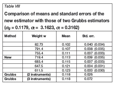
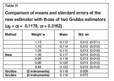
The preceding three tables show the excellent performance of the new estimator compared to the Grubbs estimators in a range of practically representative situations. The Equation [23] for the standard error of the new estimator seems also to produce standard error estimates that are close to the 'true' standard errors, i.e. those obtained from the simulated results. The following conclusions, which can be established by mathematical calculations, are also supported by the simulation results in the preceding three tables:

If σt is not excessively large compared to σg, the new estimator has smaller standard error than the three instrument Grubbs estimator. At any given sample size and value of , this superiority diminishes and will be eventually lost when σt becomes sufficiently large

If σt is large compared to σg (e.g. one order of magnitude, typically the situation in practice), the new estimator has smaller standard error than the twoinstrument Grubbs estimator. At any given sample size, this superiority diminishes and will be eventually lost when σt becomes sufficiently small (a circumstance that rarely prevails in practice)

Prior mis-specification of the ratio w₀ (weight) by as much as 15% does not lead to a bias of major significance in the estimation of σg.

Sample size determination

An important question in any gauge evaluation is how many batches to interrogate in order to reach a more or less definitive conclusion. In order to give practical content to the term definitive, notice that in checking whether or not a performance guarantee such as that the gauge error has standard deviation less than σ₀ is met, one does not simply compare the estimate of σg to the guarantee value σ0 and reject the guarantee if exceeds σ₀. Since the gauge precision is estimated from a finite amount of data, some margin of error must be allowed regarding a final pronouncement. Typically one would place an upper bound, U, on the observed value of , the estimator of σg, and require that the latter should not exceed U. In statistical terms, U is the upper limit of a, say 95%, one-sided confidence interval, (0, U) , for σg: we wish to be 95% confident that σg does not exceed the value U. Consider, for instance, the measurement of specific energy which varies on a batch-to-batch basis with a standard deviation σt = 1.5 MJ/kg and a sampling and analysis standard deviation known from past experience to be σt ≈ 0.6 MJ/kg. The vendor's guarantee is that the standard deviation of the gauge error does not exceed σt = 0.2 MJ/kg. How many batches (n) are required to come to an equitable decision if one is willing to accept the guarantee only if 0.4?

From Equation [23] a 95% one-sided confidence interval for σg has upper bound

Setting = σ0 = 0.2, U = 0.4, and σe = σ0² = 0.04 and solving for n gives n = 34.

It is illuminating to see what results if one contemplates using the three-instrument Grubbs estimator in this case. If each reference instrument interrogates k batches of coal, the total number of assays involved is n = 2k. Assume for simplicity that the two reference instruments have the same measurement precision, namely σ_l ≈ 0.6 MJ/kg. The standard error of the Grubbs three-instrument estimator of σg is then

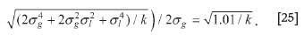
Therefore, in this case,

Setting U = 0.4 and solving gives k = 69, that is, n = 2k = 138, about double the number required by the new estimator. This example serves again to illustrate the potential savings to be had from implementing the new method when reasonably accurate prior information on gauge and quality variances are available.

 

Detection of bias

The method of estimating precision described in the preceding section allows for, and automatically takes account of, a constant bias such as that represented by the term α in Equation [14]. A more pernicious type of bias, namely a bias of scale, must also be considered in the context of a two instrument setup. In an evaluation of an online gauge one would, presumably, test for bias before proceeding to an estimation of the instrument precision-there is little interest in an instrument which produces an incorrect value with high precision. To incorporate scale bias into the analysis we replace Equation [14] by

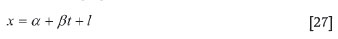
Again, Equation [27] does not imply that the sampling and analysis operation is responsible for the scale bias-bias is defined relative to what the analyser is reporting as the 'true' coal quality. Only a separate bias test on the sampling system could establish which of the two instruments is responsible for any bias that may be detected.

A glance at Equation [27] suggests estimating β by least squares from a regression of x (sampling and analysis result) on t (true coal value). However, since t is unknown and since is typically quite small, it is natural to consider using y in Equation [13] as a surrogate for it. The least squares estimator of β in Equation [27], obtained by regressing x on y, is

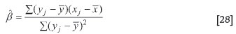
Now is in fact not an estimator of β at all. Instead, it estimates

rather than β (recall the definition of w0 from [16]. The situation is ameliorated by using instead the adjusted estimator

where w is the prior estimate of w0. Then estimates φβ, where

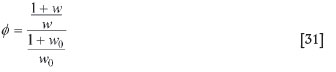
rather than β. In most cases of practical import, that is when w0 is a relatively large number, the factor φ is numerically quite close to 1 even if w over- or underestimates the true value w0 by as much as 15%. Suppose, for instance, w0 = 10. Using a 15% overestimate of w0, namely w = 11.5, gives φ = 0.988, while using a 15% underestimate, w = 8.5, gives φ = 1.016. Thus in these two circumstances estimates 0.998 × β and 1.016 × β respectively (while the unadjusted least squares estimator β estimates 0.91 × β). In general, therefore, it is not a serious mis-statement to say that in Equation [30] estimates β. Setting X = x × (1 + w)/w one sees that the adjusted estimator is the least squares estimate of slope in a regression of X on y. In most circumstances of practical relevance, therefore, one can check for scale bias by applying ordinary least squares methods to estimate the regression of X on y. If scale bias is present, cannot be estimated directly by any of the methods discussed in this paper.

 

Summary and conclusions

A new statistical method for estimating the precision of an online gauge that requires only one set of comparative laboratory analysis results has been developed. The method is substantially cheaper to implement than the often used three-instrument Grubbs estimation method, which requires two independent sets of comparative sampling and laboratory analysis results. The method is also substantially more efficient then the two-instrument Grubbs method. The efficacy of the new method has been illustrated via Monte Carlo simulation. Examples have been given that demonstrate the calculation of the new estimate and its standard error. Calculations required to determine ahead of time the number of samples required to estimate gauge precision with a pre-specified standard error have also been shown. Finally, it has been shown how the data might be used to check the gauge calibration for biases. The method is applicable only if reasonably accurate prior information is available in respect of the coal and gauge variances.

 

References

1. GRUBBS, F.E. On estimating precision of measuring instruments and product variability. Journal of the American Statistical Association, vol. 43, 1948. pp. 243-264.         [ Links ]

2. ROSE, C.D. Methods for assessing the accuracy of on-line coal analyzers. Journal of Coal Quality, vol. 10, 1991. pp. 19-28.         [ Links ]

3. ISO 15239:2005 - Evaluation of the Measurement Performance of On-line Analysers. Geneva.         [ Links ]

 

 

Paper received Dec. 2010; revised paper received Jun. 2011.

 

 

© The Southern African Institute of Mining and Metallurgy, 2011. SA ISSN 0038-223X/3.00 + 0.00.