SPECIAL EDITION

 

A stochastic programming approach for solar salt production process optimisation

 

 

R. Coetzer^*; C. Bisset

School of Industrial Engineering, North-West University, Potchefstroom, South Africa

 

 

---

ABSTRACT

The solar salt mining process involves collecting salt water from the sea and trapping it in an interlinked network of shallow ponds where the sun evaporates most of the water. As soon as the brine reaches its saturation point, salt crystallisation occurs. Several factors influence this mining process, each with a degree of variability that results in a risk factor owing to uncertainty. This study proposes a two-stage stochastic programming model, called 'a recourse model', that maximises salt crystallisation while providing solutions that are hedges against uncertainty. First, the theoretical background on optimisation theory is provided, followed by an overview of the mining processes. Second, the recourse model is verified and validated using historical data and comparing the results with its deterministic counterpart. The main contribution of this study is the formulation of the recourse model and the value that this approach adds when dealing with uncertainty in any decision-making process.

---

OPSOMMING

Die sonsoutmynproses behels die versameling van soutwater uit die see en vasvang in 'n onderling gekoppelde netwerk van vlak damme waar die son die meeste van die water verdamp. Sodra die pekelwater sy versadigingspunt bereik, vind soutkristallisasie plaas. Verskeie faktore beïnvloed hierdie mynbouproses, elk met 'n mate van veranderlikheid wat 'n risikofaktor tot gevolg het as gevolg van onsekerheid. Hierdie studie stel 'n twee-stadium stogastiese programmeringsmodel voor, genaamd ''n beroepsmodel', wat soutkristallisasie maksimeer terwyl oplossings verskaf word wat teen onsekerheid verskans word. Eerstens word die teoretiese agtergrond oor optimeringsteorie verskaf, gevolg deur 'n oorsig van die mynbouprosesse. Tweedens word die beroepsmodel geverifieer en bekragtig deur historiese data te gebruik en die resultate met sy deterministiese eweknie te vergelyk. Die hoofbydrae van hierdie studie is die formulering van die beroepsmodel en die waarde wat hierdie benadering byvoeg wanneer onsekerheid in enige besluitnemingsproses hanteer word.

---

 

 

1. INTRODUCTION

Solar salt mining involves collecting salt water from the sea and trapping it in an extensive network of interlinked dams where water evaporation occurs. Subsequently, the brine is placed in evaporation pans where salt precipitation occurs, and the salt is mined. The dams are 200 mm deep, with room for 200 mm of extra water. Shallow dams with a large surface area maximise the brine (salt water) evaporation as it navigates through the network of dams. The brine in each dam has a higher specific gravity (SG) than in the previous dam. Specific gravity is determined by the density of a reference material at some temperature, divided by the density of pure distilled water at 0 °C, and is a unitless number [1].

About 80% of the original water is lost in passing through the system. The dams are positioned in such a way as to minimise the number of pumps that are required to transport the water, thereby reducing operational costs. The flow of water is primarily controlled with rudimental slues and gravity. After passing through the network of dams, the brine flows into the salt pans, where salt crystallisation occurs. The tempo of salt crystallisation increases as the SG of the water increases. Multiple other minerals are present in the water. Figure 1 plots the chemical composition of the minerals in the water at various SG levels.

 

 

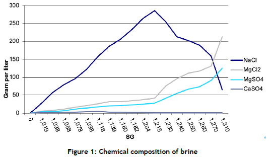
When the salt (NaCl) concentration is higher than 250 g/l, the tempo of crystallisation is optimal. As soon as the salt concentration decreases, the concentration of impurities such as magnesium sulphate (MgS0₄) and magnesium chloride (MgCl₂) rapidly increases. This contaminates the salt and lowers the quality of the final product. Maintaining a constant SG of between 1215 kg/m³ and 1240 kg/m³ in the salt pans is essential; draining and replacing the water is also necessary.

It takes roughly 18 months for enough salt to crystallise in a pan before harvesting can begin. For this reason, the system must be balanced, meaning that there is enough brine higher up in the system at an SG level slightly lower than 121 5 kg/m³. This ensures that crystallisation only occurs in the salt pans where the salt can be harvested.

The mine's planning is currently based on historical data. This planning method has a significant margin of error, leading to possible supply uncertainty from the salt pans. Given the system's sensitivity, there is a high risk of unbalancing it while optimising the salt production process. In the event of a salt shortage, the factory would be unable to satisfy demand. An unreliable business would suffer a loss in sales and customers, which would immediately have an impact on the company's revenue; and a revenue loss would severely harm numerous aspects of the company [2].

It is evident that the salt mining process is complicated and is badly affected by uncertainty. The network of evaporation dams and crystallisation pans forms a delicate system that must be balanced. Various uncontrollable weather factors significantly affect the system, and must be monitored daily. All of these factors play a role in the supply capacity of the system, leaving a significant margin of uncertainty. The salt mine's supply does not currently meet the factory's demand.

This study aims to address the problem by proposing a two-stage stochastic programming model - that is, an optimisation model that addresses the supply uncertainty from the salt mine; and to provide future research opportunities that are based on the findings and discoveries that are documented here. This model aims to maximise the salt crystallisation while providing solutions that provide a hedge against uncertainty. The main contribution of this study is the formulation of the recourse model and the value that this approach adds when dealing with uncertainty in the decision-making process.

In Section 2 a literature study is conducted on optimisation theory and stochastic programming models; then the constraints, restrictions, and rules that govern the system's behaviour will be quantified. The two-stage stochastic programming model is formulated and proposed in Section 3. Section 4 documents the verification and validation of the model, followed by a summary and the conclusion in Section 5.

 

2. LITERATURE REVIEW

The literature study is conducted to understand the industrial engineering techniques and basic principles that are required to solve the problem described in Section 1.

2.1. Overview of optimisation theory

To deal with disruption and uncertainty, the industry must use tools while considering the business situations, difficulties, limitations, and constraints [2]. Using optimisation theory as an approach to decision-making is a repetitive process in which a model is developed and continuously tested. This allows for a simple model to be developed that captures the essence of the system or problem being addressed. After that, sophisticated complications and constraints are added. A mathematical model is a mathematical representation of a real-world system or problem with varying complexity levels.

Developing a mathematical model aims to obtain a scientific understanding of a system, evaluate the effect of change on a system, and aid in tactical and strategic decision-making [3]. The two main types of model are distinguished by the kind of outcome that is predicted. Deterministic models are formulated with a set of constants that are derived from real-world data, consider random variables, and exclude uncertainty. Generally, these random variables are derived as the mean of a data set, but they do not always accurately represent the data [4]. Various models are developed that deal with deterministic optimisation. These include, but are not limited to, linear programming (LP) and integer linear programming models (ILP). To provide more context, the standard formulation of an LP is as follows:

Maximise

subject to

and

where

Linear programming is applied in various industries such as mining [5], finance [6], manufacturing [7], and the retail industry [8]. Deterministic optimisation's counterpart, stochastic optimisation, deals with decision-making under uncertainty. These models consider uncertainty and predict a distribution of possible outcomes [9].

Various methods deal with decision-making under uncertainty. These include robust optimisation and chance-constrained and stochastic programming. This paper focuses on stochastic programming, and therefore explains it in detail.

Stochastic programming is a mathematical model for solving linear or integer programming models while considering a degree of uncertainty within parameters, and is known for "providing solutions hedged against uncertainty". The formulation of a stochastic programming model is more complicated than that of a standard LP. A stochastic programme is a set of linear programmes representing various outcomes that depend on the uncertain events that occur. A stochastic model will give an LP the optimal solution, regardless of the variables' uncertainty level. Different formulations deal with uncertainty, such as two-stage and multi-stage stochastic programming models [10]. This study focuses specifically on the two-stage stochastic programming approach. A two-stage stochastic programming model is formulated as follows:

Minimise

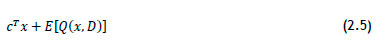
where

While solving an optimisation problem, one has access to information on which a decision is made. This is referred to as the first-stage decision. The first term (c^Tx) represents the first-stage decision, with the vector (x) being the decision variable. After this decision, a few possible outcomes may occur later, and it is impossible to know which one will influence the model's performance. Each of these outcomes is referred to as a scenario, where S = [low, medium, high], and a decision must be made that accommodates each of these scenarios. This decision is called a second-stage decision, represented by E[Q(x,D)]. The second-stage decision must be made in conjunction with the first-stage decision when it is unknown which scenario will be realised [11]. Therefore, the second-stage decision is also referred to as the expected function.

In industry, there is a wide application of two-stage stochastic programming models. For example, Liu et al. [5] proposed a two-stage stochastic programming model to allocate retrofit resources for highway bridges to provide protection against natural and human-caused hazards. Bisset [12] developed a stochastic programming model for marketing campaign optimisation. The industry context and all of the essential factors to consider when developing a recourse model are explained in the next section.

2.2. Industry context

The constraints, restrictions, and rules that govern the system's behaviour must be quantified in order to model and optimise the system. The five main factors that have the greatest influence have been identified: 1) salt water intake, 2) available evaporation and crystallisation surface area, 3) crystallisation rate, 4) brine evaporation rate, and 5) other limitations. These are explained in detail in Sections 2.2.1 to 2.2.5 below.

2.2.1. Salt water intake

The tide must be accounted for because salt water is pumped from the nearby estuary into the system. The tide affects the amount of salt present in the water. Ideally, water is only pumped at high tide. The pumps can operate for 15 hours daily to pump enough water into the system. There are two pumps, with a capacity of 750 and 650 litres per hour respectively. The salt content of the water is 14 grams per litre, as specified by the company.

2.2.2. Available evaporation and crystallisation surface area

Solar salt evaporation is relies heavily on the available surface area. The current combined area (at the primary and secondary sites) that is suitable for use as evaporation ponds and crystallisation pans is given in Table 1.

 

 

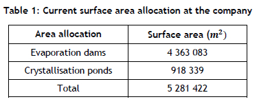
For the model, considering only the total available area is essential. For the purpose of this model, three area allocations are used: the low SG evaporation area, the high SG evaporation area, and the crystallisation area.

2.2.3. Crystallisation rate

The SG levels of the brine directly impact the salt's crystallisation rate (precipitation) and the evaporation rate that is experienced. The company's current planning system uses statistically predicted growth rates, as shown in Figure 2. The company requires that these growth rates be used for the mathematical model.

 

 

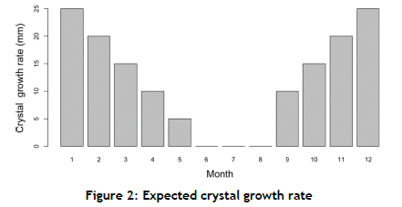
The growth rate indicates that the salt crust formed at the pan's bottom will grow by the amount indicated. The actual crystallisation rates are not constant, and depend on the weather and the management of the salt pan.

2.2.4. Brine evaporation rate

The company has a weather station with documented weather data from 1993 to 2021. One of these measured data points is the evaporation rate of brine. However, this measurement is only applicable to seawater. As the salt concentration increases in the water, the evaporation rate reduces drastically.

Figure 3 shows the monthly evaporation from 1993 to 2021. However, this does not consider the accumulative rainfall that occurs. The model derived by Glen Akridge [6] can be used with the additional recorded data points to determine more accurately the exact evaporation rates. This introduces a high level of complication to the model; but adding this to the model at a later stage is a possibility. Measuring the evaporation levels is also not an option, as each pond has a continuously variable inflow and outflow of brine.

 

 

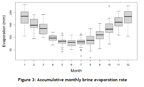
As seen in Figure 3, some years experience a higher tempo of evaporation, which is advantageous, provided that enough seawater can enter the system simultaneously. For each month, the evaporation follows a normal distribution. Therefore, each month has a distinct mean and interquartile range (IQR). This variability source dictated the system's behaviour (evaporation rate and crystallisation tempo). The company currently estimates the evaporation levels for brine with a medium SG level of 70% and a high SG level of 50% of fresh water.

2.2.5. Other limitations

Harvesting of salt can only begin once a crust of at least 300 mm has formed. A crust of 150 mm must be left behind, and cannot be harvested; this is to ensure that the harvesting machine does not strike rocks. The company uses an SG of 1.14 for the dry salt (formed as the crust) to calculate the mass of the salt formed in the crust.

The data points and the information provided and discussed in this chapter form an integral part of developing the mathematical model that addresses the uncertainty at the salt mine. The data provided and the company's assumptions must be used, as these are the model's requirements. These points provide guidance and a framework for the system's behaviour and for mathematical modelling.

 

3. MODEL FORMULATION

Formulating a recourse model consists of three parts. First, the model scenarios are described, followed by the model notation and assumptions. Last, the proposed mathematical model is formulated.

3.1. Decision-making under uncertainty: Scenario explanation

As previously mentioned, the brine's evaporation rate has a direct impact on the salt that is produced. Owing to the high level of variability in the monthly evaporation rate, the following three scenarios are derived: S = {low, medium, high}. Associated with each scenario seSis a probability p_s. Each scenario is paired with a different monthly evaporation rate for one year of production, as shown in Table 2.

 

 

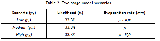
Table 2 shows the distinct scenarios that may occur, along with an assigned likelihood of occurring. The evaporation rate is determined as the mean evaporation rate for the month ± the IQR for that month, as obtained from Figure 3. The model notations are defined in Section 3.2.

3.2. Model notation

The following indices are defined:

• i e I is the index for the area allocation.

• tET is the index for periods (months).

• seS is the index for the designated scenarios.

The following decision variables are identified:

• a_; is the total area designated for the specific area i.

• ç_£ is the total amount of crystallised salt for month t.

• q_sti is the total volume of brine that flows into location i.

The following parameters are defined:

• inv_sti is the total volume of brine that flows into location i.

• sinv_st is the total amount of salt that flows into location i.

• e_stl is the total volume of fresh water that is evaporated.

The following constants are formulated:

• G_n is the SG of salt.

• G_w is the SG of fresh water.

• C_t is the crystal growth for month t.

• Τ is the total available area.

• Q_t is the maximum volume of water pumped into the system for month t.

• D is the total salt demand for one year of production.

• E_st is the evaporation tempo.

The following assumptions are made:

• The model will be applied for a period of one year t.

3.3. Proposed two-stage stochastic programming model

Maximise:

subject to:

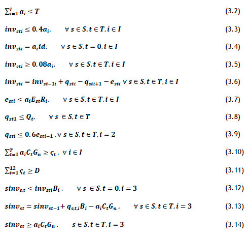
The objective function (3.1) maximises the salt yield in the first stage by allocating the optimal area for the crystallisation pans. The second stage maximises the flow of brine within the system. Constraint (3.2) ensures that the total assigned area does not exceed the available area. Constraints (3.3) to (3.6) are the parameterised set of constraints that manage the total brine volume in the network of dams. Constraint (3.7) specifies the monthly evaporation tempo for the various scenarios. Constraint (3.8) limits the total volume of water that is pumped into the system, constrained by the physical pumps that are used. Constraint (3.9) defines the brine flow to the next dam, proportional to the volume of water that is evaporated in the dam. Constraints (3.10) and (3.11) ensure that the model produces the amount of salt that the factory requires. Constraints (3.12) to (3.14) are the parameterised constraints that measure the amount of dissolved salt in the crystallisation ponds.

As mentioned earlier, this study proposes a two-stage stochastic programming model that allocates the optimal area for evaporation dams and crystallisation pans. This model is verified and validated in Section 4.

 

4. VERIFICATION AND VALIDATION

In this section the mathematical formulation of the model is verified. The results obtained by the model are validated to ensure that the model is effective and solves the underlying uncertainty problem by providing solutions that provide a hedge against uncertainty.

4.1. Verification

Section 2 identifies the essential factors to consider when formulating a recourse model, along with the stochastic programming model proposed in Section 3. The constants presented by equations (3.1) to (3.14) are critically evaluated, using IBM CPLEX (optimisation software) to verify the model. This is conducted by evaluating each constraint's impact on the model's results. It is essential to note that small-scale data is used for the verification phase to simplify the process and to make evaluation easier.

4.1.1. Objective function

The objective function is first verified without including any constraints. To assess the impact of each constraint, a baseline must be set for evaluation to occur.

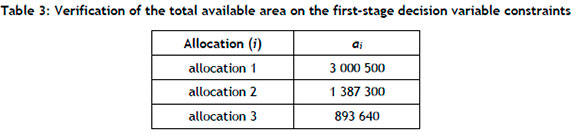
Table 3 provides the first-stage decision variables. The model yields ς = 189 885 800 kg of crystallised salt, which exceeds the demand from the factory. This is expected, since no constraints are yet considered in the model.

 

 

4.1.2. The total available area

One main limiting factor for the company is the total area available for salt production. For constraint (3.2), increasing the total available area by 20%, the model is expected to deliver an increased amount of crystallised salt, along with an increased surface area allocation for (a_i) in the first stage of the model. The results are shown in Table 4.

 

 

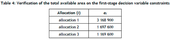
Table 4 proves that increasing the total available area by 20% increases the value of each area allocation compared with the values obtained in Table 3. Furthermore, the total number of tons of salt that is crystallised increases to a value of ς = 226 875 000. Thus the model performs as expected.

4.1.3. The total brine inventory

As demonstrated by constraints (3.4) to (3.6), the initial brine volume in the system is reduced by 50% to verify the brine inventory. The maximum capacity of brine held in the system is a significant factor to consider; the model is expected to favour increasing the brine flow. For this reason, the model likely favours allocating area to (a₁) and (a₂) rather than to (a₃). The results are illustrated in Table 5.

 

 

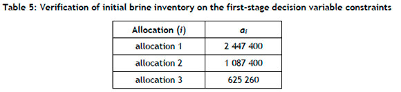
From Table 5, the total area allocated is less than that of the control model. Furthermore, the model favours (a₁) and (a₂) while barely exceeding the salt demand at ς = 129 930 200 kg. This demonstrates the importance of having a sufficient brine volume in the system. The model performs as expected.

4.1.4. Crystallisation tempo

The given monthly crystallisation tempo is decreased by 20% to verify the crystallisation constraints. Therefore, it is expected that the total salt crystallisation will be reduced. The results are shown in Table 6.

 

 

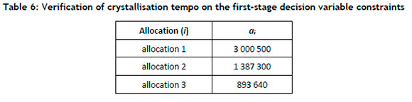
Table 6 indicates that the area allocation has remained unchanged, but that the total salt produced has decreased to ς = 151 908 200 kg. Thus the model performs as expected.

4.1.5. Individual scenario evaluation

The three distinct scenarios s eS = {low, medium, high}are differentiated by the evaporation tempo (E_st). When evaluating each scenario individually, it is expected that the salt crystallisation is lower for a low evaporation scenario, and increases for the higher scenarios. Evaluating the distinct scenarios also verifies the evaporation constraint (3.7), as this is the primary constraint being influenced. Furthermore, the area allocation is expected to correlate with the salt crystallisation. The result for each scenario is presented in Table 7.

 

 

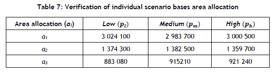
Table 7 shows that the area allocations of each distinct scenario vary from one another and from the control model, as seen in Table 6. As expected, the high scenario (p_h) also allocates a greater area for the crystallisation pans (a₃) than the medium (p_m) or the low (p_i) scenarios. The result for each scenario is presented in Table 8.

 

 

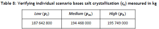
Table 8 illustrates that increased amounts of salt crystallisation occur with higher evaporation levels, according to the distinct scenarios. The distinct scenario evaluation is as expected. The second stage of the model is therefore verified.

Section 4.1 evaluates the recourse model's functionality by assessing each constraint's impact on the results. This section also aims to verify the correctness of the mathematical formulation and code. The model performs as expected in each instance.

The model is validated in Section 4.2.

4.2. Validation

Section 4.1 identified three scenarios for the stochastic model: S = {low, medium, high} evaporation rates. First, the area allocation is validated by comparing the area allocation yielded by the recourse model with the current area allocation used by the company, as seen in Table 9.

 

 

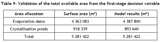
From Table 9 it is evident that the model is accurate in area allocation, as there is a clear alignment between the model's results and the current layout at the company. The model suggests that the area for evaporation dams should be slightly more than is currently used.

Second, the effectiveness of the recourse model is evaluated by comparing the results with its deterministic counterpart. As described in Section 2, a set of scenarios S = {low, medium, high} is associated with each scenario s e S as a probability p_s. The mean value scenario is also generated in this section, and is defined as S = {MV}, and associated with a probability( p_Mv).

Table 10 shows the assumed probabilities for each scenario outcome.

 

 

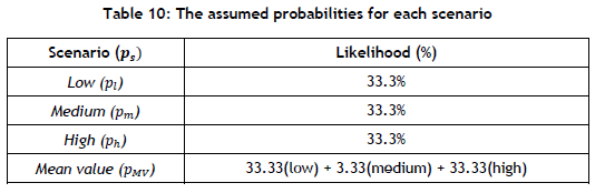
A deterministic model excludes any uncertainty in the decision-making process, and also only considers one of the scenarios S = {low, medium, high, MV} in the decision-making process, not all three concurrently. The results shown in Table 11 were obtained for each scenario.

 

 

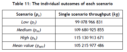
The decision-maker may assume that a low, medium, or high scenario may be realised and decided, based on only one outcome. Alternatively, the decision-maker may consider the mean of the three scenarios to make the decision.

For example, if the decision-maker assumes that a low scenario (p_;) will be realised, 990 789 668 31 kg may be obtained; whereas a high scenario (p_h ) results in a total of 115 130 913 671 kg. The same is true for the medium (p_m) and mean value scenarios (p_MV).

Basing decisions on only one scenario outcome is unreliable, since one scenario does not accommodate the outcome of an alternative scenario. This may lead to a loss in profit or of valuable opportunities. Basing decisions on taking the mean is also unreliable, since the mean plans for the average of the probabilities occurring; it does not accommodate or consider the impact of alternative scenarios occurring.

According to Higle [13], a deterministic approach is based on perfect information. The only case in which the decision-maker may assume that only a specific scenario will be realised is when enough information is available. The decision-maker can adapt after the results are known. If the decision-maker assumes a specific scenario, it may lead to a mismatch between the assumed and expected scenarios.

This analysis shows that solutions must be generated that balance the impact of all scenario outcomes. Individual scenarios and the mean value scenario do not balance this impact. This indicates that a deterministic approach does not provide solutions that provide a hedge against uncertainty.

This study proposes a two-stage stochastic programming model that allocates the optimal area for evaporation dams and crystallisation pans while providing solutions that provide a hedge against uncertainty. To demonstrate that the recourse model provides solutions that do provide such a hedge, that model's results are compared with the deterministic single scenario outcomes' results, as shown in Table 12.

 

 

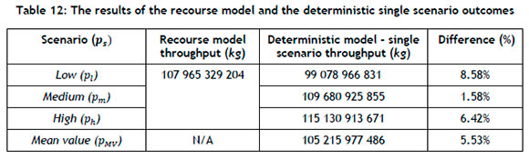
It is important to note that the stochastic model considers all three scenarios, and not the mean value. The recourse model generates a result of 107 965 329 204 kg of area allocation. Each scenario outcome is also observed.

The recourse model provides a solution that partially satisfies all three possible scenarios: low (p_i), medium (p_m), and high (p_h). If the low scenario occurs, the decision-maker can recover, since the area allocation per kg does not differ by a significant percentage. Alternatively, if the high scenario is realised, the company will not meet the demand. However, the decision-maker would retain more profit. It would also be able to recover, since the consequences are not significant as the risk of assuming one scenario outcome with its deterministic counterpart. The same principle applies to the medium scenario outcome. No outcome is guaranteed, so a resource model provides reliable solutions that will partially satisfy all possible scenarios that are identified.

The significance of a recourse model can be greater when more possible scenario outcomes are considered. A recourse model's results do not accommodate each scenario completely; however, it does allow the decision-maker to recover for any scenario outcome.

From the results discussed in this section, it is evident that the two-stage stochastic programming model makes the optimal decision and provides solutions that provide a hedge against uncertainty. The area allocation determined by the model delivers a balanced result, minimising the impact of weather uncertainty. This enables the mine to produce enough salt to meet the demand.

 

5. CONCLUSION, SUMMARY, AND FUTURE WORK

The solar salt mining process involves collecting salt water from the sea and trapping it in an interlinked network of shallow ponds where the sun evaporates most of the water. As soon as the brine reaches its saturation point, salt crystallisation occurs. Several factors influence this mining process, each with a degree of variability that results in a risk factor owing to uncertainty. These include the salt water intake, the available evaporation and crystallisation surface area, the crystallisation rate, the brine evaporation rate, and other limitations.

Given these uncertainties, this study proposes a two-stage stochastic programming model that maximises salt crystallisation per kg while providing solutions that provide a hedge against uncertainty. The first-stage decision allocates the optimal area for crystallisation pans, and the second-stage decision determines the volume of brine that flows into a specific area. The brine's evaporation rate has a direct impact on the amount of salt produced. For this reason, three scenarios are generated - S = {low, medium, high} - where each scenario is associated with a probability p_s. Each scenario is paired with a different monthly evaporation rate for one year of production.

The mathematical formulation of the recourse model is verified to ensure that the model is correctly formulated and coded in CPLEX. The effectiveness of the recourse model is validated by first determining whether the area allocation yielded by the model is similar to the current area allocation used by the company. Second, the recourse model is validated by demonstrating that a stochastic programming approach creates solutions that provide a hedge against uncertainty. The recourse model is compared with its deterministic counterpart, and the results demonstrate that the two-stage stochastic programming model does create solutions that provide a hedge against uncertainty. The area allocation determined by the model delivers a balanced result, minimising the impact or risk of weather uncertainty. This enables the mine to produce enough salt to meet the demand.

This study is only an approximation of a real dynamic system. Increasing the model's accuracy would lead to a more complex model to be solved. The current model is verified and validated for one year with three scenarios. For future research, increasing the number of scenarios is recommended. Bisset [12] applied a stochastic programming approach for marketing campaign optimisation. The computational solving time increased exponentially by increasing the number of scenarios in the model. However, various solutions are available to solve these types of complex real-life problem, including (but not limited to) the L-shape method [14], statistically based models [15], and stochastic decomposition. These types of method should be explored for future research.

 

REFERENCES

[1] R. D. Brockhaus, "Density and specific gravity," in Paint and coating testing manual, J. V. Koleske, ed. Philadelphia, PA: ASTM, 1995, pp. 289-304.         [ Links ]

[2] E. Rothberg, "How a mathematical optimisation model can help your business deal with disruption," vol. 2022, ed. Forbes.com: Forbes Technology Council, 2020. [Online]. Available: How A Mathematical Optimization Model Can Help Your Business Deal With Disruption (forbes.com)        [ Links ]

[3] D. Lawson and G. Marion, "An introduction to mathematical modelling," Bioinformatics and Statistics Scotland. [Online]. Available: https://people.maths.bris.ac.uk/-madjl/course_text.pdf (accessed 2022/07/05).         [ Links ]

[4] J. Lipscomb and D. Zalkind, "Deterministic Models for Production of Services with Stochastic Technology," Econometrica, vol. 48, no. 5, pp. 1169-1186, 1980. https://doi.org/10.2307/1912177        [ Links ]

[5] K. B. Williams and K. B. Haley, "A practical application of linear programming in the mining industry," Journal of the Operational Research Society, vol. 10, no. 3, pp. 131-137, 1959. https://doi.org/10.1057/jors.1959.16        [ Links ]

[6] W. T. Morris, "Application of linear programming to financial budgeting and the costing of funds," The Engineering Economist, vol. 5, no. 3, pp. 55-56, 1960. https://doi.org/10.1080/001379x6008546907        [ Links ]

[7] W. F. Lyle and L. L. Byars, "Linear programming for profit maximization," Journal of Dairy Science, vol. 51, no. 7, pp. 1103-1106, 1968. https://doi.org/10.3168/jds.s0022-0302(68)87135-8        [ Links ]

[8] H. Horden and C. Bisset, "Optimisation of promotions in the retail industry," South African Journal of Industrial Engineering, 2022. https://dx.doi.org/10.7166/33-3-2785        [ Links ]

[9] H. Ahmed, "Formulation of two-stage stochastic programming with fixed recourse," Britain International of Exact Sciences (BIoEx), vol. 1, no. 1, pp. 18-21, 2019. [Online]. Available: http://biarjournal.com/index.php/bioex        [ Links ]

[10] C. Liu, Y. Fan, and F. Ordonez, "A two-stage stochastic programming model for transportation network protection," Computers & Operations Research, vol. 36, no. 5, pp. 1582-1590, 2009. https://doi.org/10.1016/j.cor.2008.03.001        [ Links ]

[11] D. G. Akridge, "Methods for calculating brine evaporation rates during salt production," Journal of Archaeological Science, vol. 35, no. 6, pp. 1453-1462, 2008. doi: 10.1016/j.jas.2007.10.013        [ Links ]

[12] C. Bisset, "A stochastic programming approach for marketing campaign optimisation," Master's dissertation, North-West University, 2022.         [ Links ]

[13] J. L. Higle, "Stochastic programming: Optimisation when uncertainty matters," in Tutorials in operations research, Informs, pp. 30-53, 2005, https://doi.org/10.1287/educ.1053.0016        [ Links ]

[14] R. M. van Slyke and R. Wets, "L-shaped linear programs with applications to optimal control and stochastic programming," SIAM Journal on Applied Mathematics, vol. 17, no. 4, pp. 638-663, 1969. https://doi.org/10.1137/0117061        [ Links ]

[15] A. Shapiro, Stochastic programming by Monte Carlo simulation methods, 2000. https://api.semanticscholar.org/CorpusID-.17825017        [ Links ]

[16] J. L. Higle and S. Sen, "Stochastic decomposition: An algorithm for two-stage linear programs with recourse," Mathematics of Operations Research, vol. 16, no. 3, pp. 650-669, 1991. https://doi.org/10.1287/moor.16.3.650        [ Links ]

 

 

* Corresponding author: Ryan.coetzer@4sight.cloud
ORCID® identifiers
R. Coetzer: https://orcid.org/0009-0001-8457-4671
C. Bisset: https://orcid.org/0000-0001-5296-5945

 

 

APPENDIX A: MODEL OUTPUT

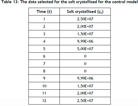
The values for the crystallised salt ç_t are set out in Table 13.

 

 

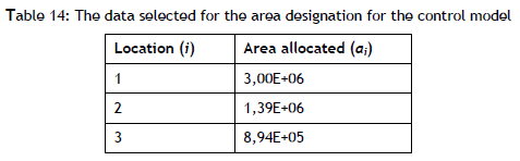
The values for the area location (a_i) are shown in Table 14.

 

 

The following data is given in Table 15:

 

 

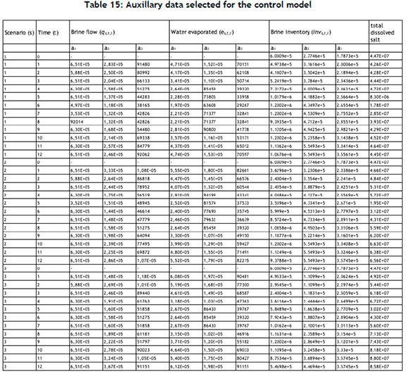
1. The values for the brine flow (q_sti) to the location (a_i)

2. The values for the water evaporated (e_sti) at each location (a_i)

3. The values for the brine inventory (inv_sti) at each location (a_i)

4. The values for the total dissolved salt (sinv_st)