Initial Investigation into Bipedal Turning: A Trajectory Optimization Study

 

 

Callen Fisher; Dean Pretorius; Nathan Weiss

Department of Electrical and Electronic Engineering, University of Stellenbosch, 7599 Stellenbosch, South Africa cfisher@sun.ac.za

 

 

---

ABSTRACT

Humans and animals leverage agility to negotiate the unpredictable environments we occupy. In order for legged robots to leave sterile lab environments, they need to be agile enough to negotiate our lives. Currently, human agility is far superior to the state-of-the-art robotic platforms. Replicating this on robotic platforms require a profound understanding of how contact events are leveraged to complete agile tasks. In line with this aim, this letter was an initial investigation into bipedal turning, to gain insight into how turning was achieved, and to identify any kinematic trends that emerged from the optimization results. This research was conducted on a simulated 10 DoF non-planar bipedal platform with point feet, and made use of a realistic friction cone, and not a linearized approximation. The mathematical model used was based on the bipedal robot currently under development. Two experiments were conducted: rapid turns with a fixed turn angle at varying speeds, and rapid turns with varying turn angles at a fixed speed. Results indicated that slip occurred 93.32% of the contact duration, and turn overshoot was present in all trajectories analyzed. Additionally, a long-time-horizon trajectory was presented to motivate the feasibility and stability of the turn trajectories studied.

Index Terms: legged robot, turning, trajectory optimization

---

 

 

I. INTRODUCTION

Much research has been done studying multi-legged locomotion [1]-[3]. However, there is stark contrast between the capabilities and agility of human locomotion compared to locomotion exhibited by the state-of-the-art bipedal robotic platforms. Humans can efficiently complete complex tasks, in an unpredictable world, and react to changes in a very agile manner. Whereas robotic locomotion is constrained to sterilized environments where simplifications, such as prescribing a fixed contact order, are used [4] and typically struggle to achieve tasks that are considered simple for humans to achieve, such as turning at speed. This paper aims at presenting a first look at how robots should turn, and identify any trends that emerge that can assist in developing future controllers.

One aspect of turning that is fairly complex to investigate, is that of friction and the foots ability to slip. Animals make use of claws to increase their friction coefficient, and humans make use of shoes and studs to improve this for certain sports, however, we still typically slip. Much of the current literature relating to turning in locomotion is focused on steady-state turns [2], [4]. These trajectories are seeded (starting point of the optimizer) using steady-state gait patterns [2] (a series of periodic steady-state gaits that veer in the desired direction of the turn). This encourages locally optimal solutions close to the initial seeded periodic gaits. Some of these articles also have infinite friction and do not allow the foot to slip [4].

Previous work by Wensing et. al. makes use of a 3D SLIP (spring-loaded-inverted-pendulum) model to generate high speed turning trajectories, which are simulated on a 3D bipedal robot [4]. The 3D SLIP model generated trajectories for the center of mass (CoM) of the bipedal robot conducting a turn. Additional controllers are implemented to ensure the CoM of the body followed this trajectory, utilizing fixed footholds which are inferred from this trajectory. This did not allow the foot to slip or enable to optimizer to select the optimal position, contact order or type of contact (stick or slip).

The 3D slip model will quickly generate feasible and accurate CoM trajectories for periodic (steady-state) motion for a number of platforms, such as the monopod, biped and quadruped. However, they do not accurately model transient motions. Additionally, these models often assume conditions that are not applicable to transient motions: such as massless legs, no foot slip, or with an implicit contact order [5]. Analysing nature, it can be seen that the dynamics present in steady-state motions are very different to those experienced during high speed and rapid turning manoeuvres.

Another approach is to make use of whole body dynamics, instead of these simplified templates. Knemeyer et. al. generated a 60° turn trajectory at 8m/s on a 3D quadrupedal robot [2]. This model is generated using three periodic gaits as the initial guess for the optimization. Using periodic gaits to seed an optimization will help guide the optimization to a feasible solution. However, it will search in regions close to the seeded periodic gaits, biasing the solution towards locally optimal results close to that periodic gait.

Another assumption that is typically assumed in the literature, is that of the polyhedral approximation of the 3D friction cone [6]. This approximation is known to underestimate the friction value, resulting in less friction force needed to initiate slipping events. Underestimating the effects thereof, reduce the reliability of results generated from employing this method. However, in this research, a method of modelling a realistic friction cone based on the Maximum Dissipation Principle using complimentarity constraints is utilized. This method describes the effects of friction and slip more accurately [7], particularly in 3D, out of plane motion.

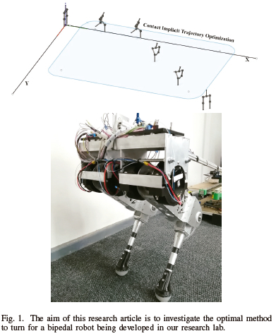
In this article, turns initiated at speeds ranging from 0.5m/s to 4.0m/s are generated for the robotic platform shown in Fig. 1. Further, with the turn speed fixed at 2.0m/s, additional turns are generated at multiple turning angles ranging from 22.5° to 90°. From these experiments, the prevalence of slip is assessed, and kinematic trends are identified. These results will assist in generating controllers for the bipedal robot that is under development.

 

 

This letter begins by detailing the trajectory optimization experiments in Section II. Section III presents the results of the experiments, which were further analysed and discussed in Section IV with the future work being presented in Section V.

 

II. METHOD

Currently a 10 degree of freedom (DoF) bipedal robot is being developed, as seen in Fig. 1. The robot utilizes four AK70-10 T-Motors, two per leg (2 DoF leg, with no ab/adduction abilities), with point feet. Throughout this paper, trajectories were generated for this robot, utilizing realistic masses and inertia's, which were estimated in CAD software. As these trajectories will eventually be executed on the robotic platform, an accurate friction cone was utilized [7], and the optimizer could pick the foot contact order and type (stick or slip), instead of enforcing it.

Trajectory optimization is an algorithmic tool that finds trajectories as solutions to mathematical problems, which are subject to a set of constraints, while minimizing an objective function. Optimization was achieved by varying a set of decision variables between bounds, and constraints, until an optimal solution was found [8]. All trajectory optimization experiments referenced in this letter were modelled in Python, using the Pyomo library, and solved using the IPOPT Solver [9]-[12].

To gain an initial insight into how a bipedal robotic platform turns, a set of rapid turns were generated using trajectory optimization methods. Furthermore, additional trends and an analysis of slip was conducted to gain further insight into rapid turning. In order to motivate the feasibility of these rapid turn trajectories, a full (long-time-horizon [5], [13] ) trajectory of the robot was generated, shown in Fig. 1, which included acceleration from rest, periodic steady-state steps, a turn trajectory and deceleration back to rest.

Due to the complexity of the long-time-horizon trajectories, the problem was broken into smaller tasks (acceleration, steady-state, turn and deceleration tasks) and optimized separately. These fragmented trajectories were then "stitched" together to form a long-time-horizon trajectory and analysed as shown in Fig. 2. This reduced the complexity of the optimization problem while increasing the accuracy of the full trajectory [5].

 

 

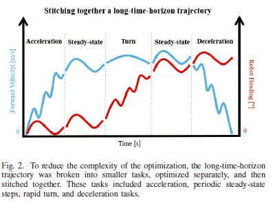
Initially, periodic steady-state trajectories were generated for each investigated speed and formed the base of the longtime-horizon trajectories. Acceleration trajectories were then generated from rest to the apex of the steady-state gait. Similarly, deceleration trajectories were generated from the apex of the steady-state gait to the rest position. Finally, trajectories conducting rapid turns were generated. These trajectories were bound to start at the apex of a steady-state gait and constrained to end at the apex of the steady-state gait (with the final heading angle offset, and the final velocity vector rotated, from the sagittal plane to the desired direction according to the turn angle).

In the following subsections the dynamics, model parameters, objectives, constraints, and problem set-up are described.

A. Dynamics and Parameters

The biped robot that was under development is shown in Fig. 1 and consists of two, two link legs, with a wide hip, and a torso. All links were modelled as solid cylindrical tubes rotating around their respective inertia axes, with parameters taken from CAD designs. Additionally, each leg consisted of a hip and knee actuator (located at the hip), resulting in four active DoF, two per leg. The generalized coordinates of the robot were:

where the first 6 generalized coordinates in q were the DoF of the body, 3 degrees of rotational freedom, and 3 degrees of translational freedom, allowing it to freely move in 3D space. This was followed by the two active DoF for each leg (using absolute angles). The model did not contain any ab/adduction DoF. This constrained the applied torque of the motors, t, around the y-axis of their respective inertia axes. The robot feet were also modelled as point contacts.

Euler-Lagrange dynamics were used to describe the equations of motion for the non-planar system. These dynamics, in the form of the manipulator equation, were implemented as:

where M(q) was the mass matrix, C(q, q) described the Kinetic Coriolis forces, and G(q) described potential gravitational forces. A(q) and B were used to map the motor torques applied to the revolute joints, t, and external ground reaction forces, A, to q [14]. This research made use of a μ =1, as the robot foot was a silicone dome, which has a coefficient of friction of 1 in many cases.

B. Constraints

Transient motions are notorious for being complex, and characterised by discontinuous dynamics and unpredictable contact events. Therefore, constraints were implemented to aid the solver in finding kinematically feasible solutions. These constraints and techniques are further described below.

1) Discretization: The trajectories generated in this experiment were all discretized to N = 100 nodes. Trajectories from the 4.0m/s experiments proved an exception to this, and required N = 150 nodes to generate an optimal trajectory. In order to provide the solver with added flexibility to model intermittent contact events, a variable time-step was employed, such that:

This allowed the duration of a discretized time-step, h_i with i e[1,N], to vary between 10% and 200% of a master time-step, h_M. h_M was used to describe a ratio between an approximated time needed to complete the task, T, and the number of nodes the trajectory was discretized to, such that h_M = . T was experimentally tuned for each velocity.

Three-point collocation methods were used to further discretize q using third order Radau polynomials and Runge-Kutta integration methods, increasing the accuracy of the results while keeping the problem computationally tractable [15].

2) Contact Implicit Trajectory Optimization: In order to fully investigate non-intuitive transient motions, a fixed contact order was not prescribed. Instead, contact implicit trajectory optimization techniques were used to give the optimizer freedom to determine the optimal contact order and type (stick or slip) for the given tasks. These methods have been proven to be vital in studying rapid locomotion [6], [15].

All contacts were modelled as inelastic collisions, on a contact surface with a uniform coefficient of friction, μ = 1.0 (due to the silicone foot), while adhering to Coulomb's law of dry friction [16]. To study the slip required to conduct rapid turning, the contact model described in [7], equations (4) to (7), were used. Here, the Maximum Dissipation Principle was used to accurately determine the direction of applied friction, while satisfying Coulomb's law.

Unfortunately, this required complimentarity constraints that are notorious for being computationally intractable. Therefore, e-relaxation schemes [17], [18] were applied to assist in solving these constraints, along with three-point collocation methods to increased the accuracy [15] of the solution as follows:

Here, a_ij and β_ij described the complimentarity variables discretized to the i^th node and the j^th collocation point. e described a relaxation parameter used to satisfy the complimentarity constraints within an acceptable tolerance (see Section II-D for more details on the tolerance value). These complimentarity variables were summed across the collocation points and the complimentarity was solved at individual node points [15].

3) Motor Model: In order to ensure the generated trajectories could work on the robotic platform, a linear motor model was implemented. This constrained the applied motor torques as a function of the relative velocity of the joint as shown:

where T_i was the applied motor torque, and uj_i was the relative joint speed, at the i^th time-step. Furthermore, T_max and w_max described the respective stall torque, and no-load speed, for the motor [5], [19]. These parameters were determined from the data-sheet of the motor used on the robotic platform (T-Motor AK70-10).

4) Average Velocity: To generate the steady-state trajectories at specified speeds, an average velocity constraint was enforced. The constraint was implemented as follows:

where x_N was the final x position (x₀ was the initial position and was set to zero) and tt_N was the final time of the periodic steady-state trajectory (with tt₀ being the initial time and was set to zero). v_avg was the desired average velocity constant, which was varied between 0.5m/s and 4.0m/s.

5) Initial and Terminal Conditions: As the long-time-horizon trajectory was split into smaller tasks, the initial and final conditions varied according to the task being optimized.

• Steady-state Trajectories: The steady-state trajectory was generated first, as it was required for the initial/terminal constraints of the other tasks. In order to achieve this, the initial pose was left unspecified, except that is was constrained to the origin of the Cartesian plane and the vertical velocity, z = 0.0m/s, and acceleration z = -9.81m/s², was fixed. This pose described the apex of the steady-state gait. Periodicity was enforced by constraining the initial conditions to equal the final conditions, except for the x variable, which allowed the robot to travel forward. The desired velocity was enforced as described in Section II-B4. This allowed the optimizer to find an optimal initial and final pose along with a periodic steady-state trajectory.

• Acceleration Trajectories: The initial conditions were set to start at rest, with all joints stacked vertically (robot standing vertically, with zero motion), at the origin of the Cartesian plan. Whereas, the final conditions were constrained to equal the apex pose of the steady-state trajectory (excluding the x variable). This allowed the robot to accelerate from rest into the periodic gait.

• Deceleration phase: Similarly, the initial conditions of the deceleration phase was constrained to equal the apex pose of the steady-state trajectory. The terminal conditions were set to stop the robot in a rest position (excluding the x variable). This allowed the robot to decelerate from the steady-state gait back to rest.

• Rapid turn: The initial conditions were set to start at the origin, in the apex pose of the steady-state trajectory. The final conditions were constrained to the same apex pose of the steady-state trajectory, however, the final yaw and velocity vector was offset by the desired turn angle, S_Turn. This allowed the robot to start and end in a periodic gait while implementing a turn manoeuvre.

C. Objective Function

Due to the complexity of the desired motions, a combination of two objective functions were implemented in these experiments. Minimum time, J_time, and minimum torque, J_torque, cost functions were implemented in tandem and integrated in the e-relaxation techniques:

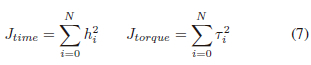
where t_i² represented the square of the individual motor torques at the i^th node, in order to penalize positive and negative torque. Additionally, h_i represented the time-step duration of the i^th node.

D. Solver Setup and Optimal Solutions

In order to successfully search the solution space, q, q, and q were initialised using randomized seeds interpolated between their respective variable bounds. Variable bounds were selected to ensure kinematic realisation of the robot (for example, the range of motion of the hip and knee were enforced with bounds), with other bounds used to restrict the search space (for example, the X position of the robot was limited from 0m to 5m), without ruling out non-intuitive solutions. Whereas the rest of the optimization variables, t and A, were initialised to 0.01 [13].

Additionally, e-relaxation schemes were used to iteratively solve the model (see equation (4)). For the first iteration, e was set to 1000, and the objective function set to a constant 1 . 0 (looking for a feasible solution to improve the initial seed, and not an optimal solution in terms of the cost function). Thereafter, the objective was set to a minimum time cost function, J_time, and e was reduced by a factor of 10 for each iteration of the optimization. As soon as an infeasible solution was returned, the respective seed was discarded and the solve process reset. The advantage of this method was that after the first successful solve (with the random seed), the optimizer was warm started with the previous iterations trajectory, and a new e value, which sped up the solve time.

However, it was noticed that the minimum time cost function guided the solution towards a local minima that produced very erratic and infeasible trajectories that violated the conservative motor model. Therefore, once e =1.0, the objective function was changed to a minimum torque objective, J_torque, to smooth the trajectories and find a more torque sensitive solution. After 8 successful iterations, and e = 1E - 4, all complimentarity constraints were considered satisfied within an acceptable tolerances.

 

III. EXPERIMENTS AND RESULTS

Initially, steady-state, acceleration, and deceleration trajectories were generated as described in Section II. These trajectories were generated at multiple velocities, such that v_avg ε{0.5,1.0, 2.0, 4.0}m/s.

Thereafter, two investigations were conducted into rapid turning. First, rapid turning was conducted at each velocity, v_avg, with a fixed turn angle, 0_Turn = 45°. Secondly, rapid turn optimizations were conducted at a fixed velocity, such that v_avg = 2.0m/s, and multiple turn angles, such that O_Turn e{22.5°, 30°, 45°, 60°, 90°}.

Finally, optimal trajectories for each phase described in Section II-B5 were stitched together to generate a longtime-horizon trajectory, in which the robot started at rest, accelerated to a steady-state velocity, performed a rapid turn, proceeded with a steady-state velocity and then decelerated back to rest.

These results are split into three sections, and detailed below:

A. Turning at varying speeds

In Table I, the characteristics of the trajectories conducting a rapid turn with a fixed turn angle, 0_Turn = 45°, at multiple speeds, such that v_avg E{0.5, 1.0,2.0,4.0}m/s, are presented. Five rapid turn trajectories were generated at each speed of interest.

 

 

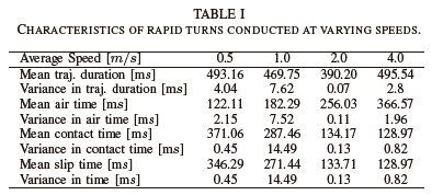
As the speed of the robot increased, a decreasing trend was noticed in the average contact time relative to the average trajectory duration. Contact occurred 75.24% of the trajectory duration when the robot was turning at 0.5m/s; 61.19% at 1.0m/s; 34.38% at 2.0m/s; and 26.02% at 4.0m/s.

Additionally, an increasing trend was noticed in the amount of slip relative to the average contact time. Slip occurred 93.32% of the average contact duration at 0.5m/s; 94.42% at 1.0m/s; 99.65% at 2.0m/s; and 100% at 4.0m/s.

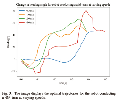
In Fig. 3, the optimal trajectories for the change in heading angle of the robot conducting 45° rapid turn at varying speeds can be seen. An overshoot in the turn angle was present in all of the turns, and the magnitude of the overshoot was noticed to increase proportionally to the speed of the robot. For turns conducted at 0.5m/s an overshoot of 0.25° was observed; 10.07° at 1.0m/s; 21.29° at 2.0m/s; and 35.80° at 4.0m/s.

 

 

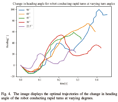
B. Turning at varying degrees

In Table II, the characteristics of the trajectories conducting rapid turns at varying turn angles, 0_Turn € {22.5°, 30°, 45°, 60°, 90°}, at a fixed speed, V_avg = 2.0m/s, were presented. Five rapid turn trajectories were generated at each turn angle of interest. The characteristics relevant to 45^° turns were displayed in Table I under the 2.0m/s column.

 

 

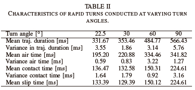
A flat trend was noticed in the average contact time relative to the average trajectory duration, ranging between 31.00% and 41.15%. Similarly, a flat trend was noticed in the average amount of slip relative to the average contact duration, ranging between 97.75% and 100.0%. An increasing trend was noticed in the average trajectory duration: 331.67ms at 22.5°; 353.46ms at 30°; 390.20ms at 45°; 484.77ms at 60° ; and 566.43ms at 90^°.

However, a relatively flat trend was noticed in the amount of overshoot relative to the turn angle. An overshoot of 4.45^° was observed for a 22.50° turn; 24.07° for a 30° turn; 13.84° for a 45° turn; 14.48° for a 60° turn; and 9.84° for a 90° turn. Fig. 4 displays the optimal trajectories for the change in heading angle of the robot conducting a rapid turn, of varying degrees, at 2.0m/s.

 

 

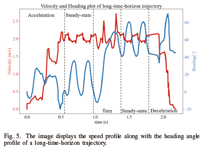
C. Long-Time-Horizon Trajectory

Typically, rapid turns are conducted once the robot has reached a desired speed and needs to rapidly change its direction. To make the results presented in this research more realistic, an optimal 45° turn was stitched onto acceleration, deceleration, and steady-state trajectories to generate a longtime-horizon trajectory. Fig. 5 shows the speed and the heading angle profile of this long-time-horizon trajectory. The turn was only initiated after an acceleration trajectory and two steady-state periodic steps (0.86s into the trajectory). During the turn phase, the heading angle was offset as specified. Finally, the trajectory concludes with two more steady-state periodic steps, and a deceleration trajectory. The total trajectory duration was 2.34s long.

 

 

IV. DISCUSSION AND CONCLUSION

In this letter, the presence of slip is shown to be significant in performing turning manoeuvres. Comments on the kinematic trends that emerged during these turning manoeuvres are also made. Two different trajectory optimization experiments are presented in this research, namely: rapid turning at varying degrees with a fixed speed, and rapid turning to a set degree at varying speeds.

Results shown in Section III are significant as they show an initial insight into how a bipedal robot should perform turning manoeuvres, especially concerning slip. These results show the importance of modelling friction as well as allowing the slip condition to occur (through the use of contact implicit methods). Table I, and Table II, both indicate significant amounts of slip needed for conducting a rapid turn at all speeds and turn angles investigated. on average, slip occurred at least 93.32% of the contact time while conducting 45° rapid turns at all speeds investigated. Similarly, slip occurred at least 97.52% of the contact time while conducting rapid turns at 2m/s at all turn angles investigated. Additionally, a long-time-horizon trajectory is generated to show that the robot (in simulation) is capable of accelerating to, and decelerating from a steady-state gait, as well as being able to perform a rapid turn from the steady-state gait.

Further, this research set out to comment on kinematic trends noticed when conducting rapid turns. Fig. 3, and Fig. 4, provide evidence of turn overshoot for all optimal results displayed. However, it is also noted that for rapid turns conducted at 2.0m/s with varying turn angles, the overshoot is approximately the same magnitude, ranging between 5.26° and 14.12°. Whereas, the overshoot increased with the speed for 45^° turns conducted at varying speeds. similar comments can be made when analysing the initial undershoot for all turns. This is inline with the observation made by Perkins et. al., that the overshoot is proportional to the speed of the turn, and not the degree of the turn [3].

 

V. FUTURE WORK

Future work involves implementing these trajectories onto the bipedal robot shown in Fig. 1, which is currently under construction. This will involve developing controllers to ensure that the robot accurately tracks the generated trajectories. some of the parameters in the optimizer may have to be tweaked, should the developed robot drastically differ from the mathematical model used.

 

REFERENCES

[1] P. M. Wensing, Optimization and control of dynamic humanoid running and jumping. The Ohio State University, 2014.

[2] A. Knemeyer, S. Shield, and A. Patel, "Minor change, major gains: The effect of orientation formulation on solving time for multi-body trajectory optimization," IEEE Robotics and Automation Letters, vol. 5, no. 4, pp. 5331-5338, 2020.

[3] A. D. Perkins, Control of dynamic maneuvers for bipedal robots. Stanford University, 2010.

[4] P. M. Wensing and D. E. Orin, "3d-slip steering for high-speed humanoid turns," in 2014 IEEE/RSJ International Conference on Intelligent Robots and Systems, 2014, pp. 4008-1013.

[5] C. Fisher, C. Hubicki, and A. Patel, "Do intermediate gaits matter when rapidly accelerating?" IEEE Robotics and Automation Letters, vol. 4, no. 4, pp. 3418-3424, 2019.

[6] M. Posa, C. Cantu, and R. Tedrake, "A direct method for trajectory optimization of rigid bodies through contact," The International Journal ofRobotics Research, vol. 33, no. 1, pp. 69-81, 2014.

[7] D. Pretorius and C. Fisher, "A novel method for computing the 3d friction cone using complimentary constraints," in 2021 International Conference on Robotics and Automation (ICRA), 2021.

[8] M. Kelly, "An introduction to trajectory optimization: How to do your own direct collocation," SIAM Review, vol. 59, no. 4, pp. 849-904, 2017.

[9] G. Van Rossum and F. L. Drake, Python 3 Reference Manual. Scotts Valley, CA: CreateSpace, 2009.         [ Links ]

[10] W. E. Hart, J.-P. Watson, and D. L. Woodruff, "Pyomo: modeling and solving mathematical programs in python," Mathematical Programming Computation, vol. 3, no. 3, pp. 219-260, 2011.

[11] W. E. Hart, C. D. Laird, J.-P. Watson, D. L. Woodruff, G. A. Hackebeil, B. L. Nicholson, and J. D. Siirola, Pyomo-optimization modeling in python, 2nd ed. Springer Science & Business Media, 2017, vol. 67.

[12] A. Wachter and L. T. Biegler, "On the implementation of an interior-point filter line-search algorithm for large-scale nonlinear programming," Mathematical programming, vol. 106, no. 1, pp. 25-57, 2006.

[13] C. Hubicki, M. Jones, M. Daley, and J. Hurst, "Do limit cycles matter in the long run? stable orbits and sliding-mass dynamics emerge in task-optimal locomotion," in 2015 IEEE International Conference on Robotics and Automation (ICRA). IEEE, 2015, pp. 5113-5120.

[14] R. Tedrake, "Underactuated robotics: Algorithms for walking, running, swimming, flying, and manipulation (course notes for mit 6.832)," Downloaded in May, 2020. [Online]. Available: http://underactuated.mit.edu/

[15] A. Patel, S. L. Shield, S. Kazi, A. M. Johnson, and L. T. Biegler, "Contact-implicit trajectory optimization using orthogonal collocation," IEEE Robotics and Automation Letters, vol. 4, no. 2, pp. 2242-2249, 2019.

[16] D. Stewart and J. C. Trinkle, "An implicit time-stepping scheme for rigid body dynamics with coulomb friction," in Proceedings 2000 ICRA. Millennium Conference. IEEE International Conference on Robotics and Automation. Symposia Proceedings (Cat. No. 00CH37065), vol. 1. IEEE, 2000, pp. 162-169.

[17] D. Ralph* and S. J. Wright, "Some properties of regularization and penalization schemes for mpecs," Optimization Methods and Software, vol. 19, no. 5, pp. 527-556, 2004.

[18] T. Hoheisel, C. Kanzow, and A. Schwartz, "Theoretical and numerical comparison of relaxation methods for mathematical programs with complementarity constraints," Mathematical Programming, vol. 137, no. 1-2, pp. 257-288, 2013.

[19] M. Haberland and S. Kim, "On extracting design principles from biology: Ii. case study-the effect of knee direction on bipedal robot running efficiency," Bioinspiration & biomimetics, vol. 10, no. 1, p. 016011, 2015.

 

 

The authors would like to thank the NRF (grant number 129830) and Sub Comm B for funding this research.

 

 

Callen Fisher received his PhD in the department of Electrical Engineering at the University of Cape Town in 2021. Callen is now a senior lecturer at Stellenbosch University and is currently focused on legged robotics in extreme environments.

 

 

Dean Pretorius received his MEng in the department of Electrical Engineering at Stellenbosch University in 2022. Dean is now a researcher at the CSIR and is currently focused on IOT devices in the mining industry.

 

 

Nathan Weiss recently submitted his MEng in Electrical and Electronic Engineering at Stellenbosch University. He has recently entered the job marked.