Low Complexity Deep Learning-Assisted Golden Code Sphere-Decoding with Sorted Detection Subsets

 

 

Bhekisizwe Mthethwa^I ; Hongjun Xu^II

^ISchool of Engineering, University of KwaZulu-Natal, Durban 4041, South Africa. (email: tshomie2020@yahoo.com). Member, IEEE
^IISchool of Engineering, University of KwaZulu-Natal, Durban 4041, South Africa. (email: xuh@ukzn.ac.za), Member, IEEE

 

 

---

ABSTRACT

Golden code is a space-time block coding (STBC) scheme that has spatial multiplexing gain over the Alamouti STBC which is widely used in modern wireless communication standards. Golden code has not been widely adopted in modern wireless standards because of its inherent high detection complexity. However, detection algorithms like the sphere-decoding with sorted detection subsets (SD-SDS) have been developed to lower this detection complexity. Literature indicates that the SD-SDS algorithm has lower detection complexity relative to the traditional sphere-decoding (SD) algorithm, for all signal-to-noise ratio (SNR) values. The SD-SDS algorithm exhibits low detection complexity at high SNR; however, at low SNR the detection complexity is higher. We propose a deep neural network (DNN) aided SD-SDS algorithm (SD-SDS- DNN) that will lower the Golden code's SD-SDS low SNR detection complexity, whilst maintaining the bit-error-rate (BER) performance. The proposed SD-SDS-DNN is shown to achieve a 75% reduction in detection complexity relative to SD-SDS at low SNR values for 16-QAM, whilst maintaining the BER performance. For 64-QAM, the SD-SDS-DNN achieves 99% reduction in detection complexity relative to the SD-SDS at low SNR, whilst maintaining the BER performance. The SD-SDS-DNN has also shown to achieve low detection complexity comparable to that of the Alamouti linear maximum likelihood (ML) detector for a spectral efficiency of 8 bits/s/Hz. For a spectral efficiency of 12 bits/s/Hz, the SD-SDS-DNN achieves a detection complexity that is 90% lower than the Alamouti linear ML detector.

Keywords: Index Terms: Alamouti, deep learning, Golden code, space-time coding, sphere-decoding.

---

 

 

I. Introduction

WITH the ever-increasing demand for higher data transmission rates and link reliability for wireless radio access networks (RAN), because of increasing real-time and mission-critical applications, it becomes necessary to research and develop wireless schemes that can provide high spectral efficiency, good link reliability, and low detection complexity. Multiple-input multiple-output (MIMO) wireless techniques can deliver on these requirements through space-diversity and spatial multiplexing. Space-time block coding (STBC) schemes such as Alamouti [1], uncoded space-time labeling diversity (USTLD) [2], and Golden code [3] provide time-diversity over and above space diversity. These schemes further improve wireless link reliability over MIMO wireless channels. Of the three STBC schemes, Golden code is the only full-rate, full-diversity wireless scheme, whilst the USTLD and Alamouti are half-rate and full-diversity schemes. This paper's coding rate is defined as the number of M-QAM symbols transmitted per transmit antenna per transmission timeslot. The advantage of the Golden code is that it offers full spatial-multiplexing gain relative to the Alamouti and USTLD STBC schemes. However, Alamouti STBC has the advantage of having much lower linear detection complexity relative to the Golden code STBC scheme under block-fading wireless channels. The Alamouti optimal linear decoder has order ν (M¹) detection complexity, in block-fading channels [1], relative to the Golden code optimal detector with ν (M⁴) detection complexity. The variable M is defined as the M-QAM signal modulation order. The USTLD STBC has a coding gain advantage over the Alamouti STBC whilst achieving the same rate and diversity order [2]. However, USTLD STBC has a detection complexity of order ν (M²) since it uses joint maximum likelihood (ML) detection to decode the two transmitted symbols [2]. This USTLD STBC decoding complexity is higher than the Alamouti STBC linear detection complexity in block-fading channels. The Alamouti STBC linear decoder is shown to under-perform in terms of bit-error-rate (BER) in fast-fading channels [4] due to inter-symbol interference (ISI). The optimal detector for the Alamouti STBC scheme, in fast-fading channels, is shown in [4] to be the joint ML detector with order ν(M²) detection complexity.

Golden code STBC is a promising wireless scheme which is already incorporated into the WiMAX IEEE 802.16e standard [5]. Golden code offers spatial multiplexing gain relative to the Alamouti STBC scheme, at the expense of higher detection complexity. In modern wireless communication systems, the following standards incorporate the Alamouti STBC scheme namely, the long-term evolution (LTE) 3GPP standard [6], wireless fidelity (Wi-Fi) IEEE 802.11n [7] and IEEE 802.11ah low power Wi-Fi [8]. This makes research into the reduction of the Golden code detection complexity interesting and relevant to modern wireless communication systems. The practical application of Golden code is limited due to its high detection complexity despite its advantages of spatial multiplexity gain over the Alamouti and USTLD STBC schemes. Thus, to extract the benefits of Golden code in a practical use case, researchers have embarked on developing various detection schemes to lower the Golden code's detection complexity. Therefore, this paper particularly concentrates on the Golden code STBC due to its disadvantage of being a high detection complexity scheme. The high detection complexity has a negative implication of increasing telecommunications operator basestation processing power consumption, including that of the end-users. High complexity detection schemes may also increase end-to-end link latency if powerful detection processors are not used. An increase in link latency has detrimental effects on real-time low latency applications. Our research aims to reduce this detection complexity.

In literature, [9] develops an efficient ML detection scheme that can reduce the Golden code's detection complexity to approximately ν(M²⁵). Using dimensionality reduction of the search tree in sphere-decoding (SD), [10] manages to reduce the detection complexity to approximately ν(M^1.5). However, [10]'s side effect is that the BER performance suffers a 1dB SNR loss compared to optimal ML detection. The fast-essentially maximum likelihood (FML) detection is developed in [11] with a detection complexity of ν (M²). FML proves to be computationally intensive at higher modulation orders. In literature, a near-optimal detection algorithm called SD, with detection complexity of ν(M²), is modified in [12] by minimizing the search depth, to reduce detection complexity, using the Schnorr-Euchner strategy. It is known from literature that SD detection complexity relies on the signal modulation order and the search depth [13]. The authors in [14] further optimize the FML and SD algorithms by reducing the signal cardinality by creating detection subsets. This can further reduce the detection complexity whilst maintaining the BER performance close to that achieved by FML and SD. In [15], the authors propose SD-SDS, which has low detection complexity for Golden code at high SNR with an increasingly high detection complexity as the SNR approaches 0dB. However, it has detection complexity which is at least 1 order lower than the sphere-decoding detection subset algorithm (SD-DS) developed in [14].

Part of the challenge in [15] is that the SD initial radius is fixed per average SNR, thus at lower average SNR values, the initial radius is larger which causes a selection of many signal candidates under good instantaneous SNR conditions. This creates a high detection complexity at lower SNR values and suggests that we may need an SD initial radius calculated using the instantaneous channel conditions instead of average channel conditions. In [16], the authors develop a deep learning-based initial radius predictor that predicts an initial radius based on instantaneous channel conditions. This approach lowers the detection complexity of MIMO SD detection whilst maintaining the BER performance. Another interesting MIMO SD technique is developed by [17]. The initial radius of SD is selected and fed into a deep neural network that predicts the number of lattice points inside the hypersphere. If the predicted number of lattice points is high, then the initial radius is adjusted downwards and re-fed into the deep neural network. This is done iteratively until the number of predicted lattice points is low, at which point SD is performed with this lower initial radius that is predicted to yield a small number of lattice points inside the hypersphere. This technique yields lower detection complexity for SD. However, in our experiments, we found that [16] yields better performance than [17]. In [18], the authors propose a deep learning (DL)-aided SD for large MIMO detection. Because SD detection for large MIMO has a prohibitive computational complexity, the DL-aided SD generates a highly reliable initial candidate to accelerate the SD search for the transmitted symbols. The DL-aided SD is beneficial both from an offline training phase and online application relative to the DL-aided SD in literature. In [19], a neural network is proposed that predicts the minimum path metrics of subtrees of a SD and these predicted minimum path metrics are used for early termination in the SD search for candidates. The scheme shows significant computational complexity reduction relative to the conventional SD scheme for large MIMO, whilst exhibiting a BER performance close to the optimal detector.

Based on the literature review, we are motivated to lower the detection complexity of the Golden code SD-SDS decoder, at low SNR, for the traditional MIMO architecture. This reduction of low SNR Golden code detection complexity is important for low power wireless communications. The algorithms in [16-19] perform deep learning-aided complexity reduction in the conventional SD algorithm, for large MIMO (i.e N_t>8), except for the Golden code context with a small number of transmit antennas (i.e N_t = 2). Therefore, no literature has performed complexity reduction of the Golden code specific SD-SDS detection algorithm. The reduction in detection complexity is performed to give Golden code an edge over the Alamouti STBC scheme which is already implemented in modern wireless communication standards. Golden code has greater spectral efficiency, for the same link reliability, relative to the Alamouti STBC but at the expense of higher detection complexity which prevents it from being incorporated into broader wireless standards as an STBC scheme of choice. By embarking on lowering the detection complexity of Golden code SD-SDS, at low SNR, our paper makes the following contributions:

(i) The SD initial hypersphere radius computation is well discussed in [20-23]. However, the computation in literature is performed for a single timeslot whereas Golden code is a 2-timeslot STBC scheme. In this paper, we derive the 2-timeslot Golden code SD-SDS [15] fixed initial radius and show that this SD-SDS has an initial radius dependent only on a single timeslot, which makes the formulas discussed in [20-23] also relevant for our use case.

(ii) We present a modified version of the low complexity deep learning-based algorithm in [16]. This modified algorithm lowers the SD-SDS detection complexity at low SNR. The reason for the modification is because the algorithm in [16] is developed for a single timeslot scheme, whereas Golden code is a 2-timeslot STBC system. This has the effect of changing the DNN input vector length and thus requires us to design and train a new DNN architecture for the radius prediction. The algorithm in [16] is also developed for a very high detection complexity large MIMO (N_t > 10) SD environment whereas our scheme needs to work for a lower detection complexity traditional MIMO (N_t = 2) SD-SDS environment. Because of the lower complexity traditional MIMO SD-SDS environment, we only predict one radius at the output of the DNN unlike in [16]. To counter the error in prediction accuracy of a single radius prediction, we use the reverse of the approach in [ 17] to determine the subsequent radius predictions. This DNN algorithm is named as the SD-SDS-Radius-DNN.

(iii) SD based algorithms are generally more complex than the sub-optimal QR decomposition detector. However, under good instantaneous channel and noise conditions, the suboptimal QR decomposition detector produces M-QAM symbol estimates that are reliable. We, therefore, propose a novel DNN channel state predictor that uses the instantaneous channel conditions and received signal vectors to predict whether the low complexity suboptimal QR decomposition detector estimates are good enough to be used as the actual transmitted symbols without performing the more complex SD based search.

(iv) We also propose a low complexity detection algorithm called the SD-SDS-DNN. The proposed SD-SDS-DNN algorithm combines the high SNR low complexity benefits of the SD-SDS detector from [15], the low SNR low complexity benefits of the SD-SDS-Radius-DNN detector, and the benefits of the proposed novel DNN channel state predictor that selects between the very low complexity QR decomposition detector output and search using the SD-SDS-Radius-DNN detector.

(v) We perform the DNN architecture designs and training for the two DNNs in the paper and perform Monte-Carlo simulations of the BER and complexity analysis of the Golden code detection algorithms discussed in this paper.

The remainder of this paper is organized as follows: Section II, the system model of the paper is presented. In Section III, we present the theoretical overview of SD-SDS. In Section IV, we deal with the derivation of the Golden code 2-timeslot SD initial radius. In Section V, we present the SD-SDS deep learning algorithms. In Section VI, we perform the complexity analysis of the Golden code detection algorithms relative to SD-SDS. Section VII presents the simulation results and discussion. Section VIII concludes the paper.

Notation: Bold lowercase letters are used for vectors and bold uppercase for matrices. (. )^T (. )^H, 1.1, ||. || and ||. ||_F represent the Transpose, Hermitian, Absolute Value, Euclidean norm and Frobenius norm operations, respectively. The functions R(.) and Չ(.) are the real and imaginary components of a complex number, respectively. j is a complex number. The statistical average is represented by the expectation function E(.). The function (■)* is the complex conjugate of a complex number. The function vec(~) is a matrix vectorization function that stacks the column vectors of a matrix on top of each other to form a single column vector.

 

II. GOLDEN CODE SYSTEM MODEL

In this paper we consider a Golden code system that operates over an N_t X N_r wireless MIMO channel where N_t = 2 and N_r > N_t for optimal operation according to [24]. The parameters N_t and N_r are the number of transmit and receive antennas in the MIMO configuration, respectively. Golden code works by separating information bitstreams into 4 parallel streams. Each stream has bits packaged into log₂ M bit length words and these words are used as symbol indices to select the complex M-QAM symbols from the M-QAM complex signal constellation fl_M. This generates 4 M-QAM complex symbols that are transmitted over a wireless channel by mapping pairs of the M-QAM complex symbols onto the Golden code super symbols. The mapping of M-QAM symbol pairs onto the Golden code super symbols is performed as follows:

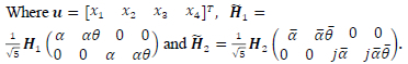
Let x₁₁,x₁₂,x₂₁ and x₂₂ be the transmitted Golden Code super symbols in which x₁₁ = and x₁₂ = and x₂₁ = and x₂₂ = . The scalar parameters a, a, 0 and 0 are defined as follows: a = 1 + j 0, a = 1+j 0, 0 = and 0 = The complex M-QAM symbols are X1, X2, X3, X4 εΩ_M, where Ω_M is an arbitrary square M-QAM signal constellation. The average M-QAM symbol power is set to 1, E (|xq|²) = l.Vq E [1:4]. These Golden code super symbols are transmitted over the air using the N_t transmit antennas with the transmit power per antenna fixed to where y is the average SNR at each receive antenna.

During wireless transmission, the Golden code transmission vector for timeslot i,i E [1:2] is set to x_t = [x_tl x_i2]^T. The wireless MIMO channel matrix for timeslot i is Hi, where Hi E CN_rxN_t is a fast frequency-flat fading wireless channel which is fully known at the wireless receiver. As a result of the wireless channel being fast fading, this means the wireless channel changes its complex channel gains for every transmission timeslot. The wireless channel fading gain is assumed to be Rayleigh distributed to mimic multipath fading without line of sight (LOS). Each entry of the wireless channel matrix Hi varies according to the independent and identically distributed (i.i.d) zero mean complex Gaussian distribution CN(0,1). The received wireless signal vector for timeslot i is given by (1)

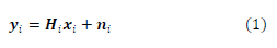
where yi EC^NrXl is the received signal vector for timeslot i and Ni EC^NrXl is the noise vector for timeslot i. Each entry of the zero mean complex Gaussian noise vector, rii, is distributed according to For this work, the detection algorithms used to detect the transmitted M-QAM symbols are the SD-SDS-DNN, SD [14] and SD-SDS [15]. These detection algorithms are evaluated against each other based on BER performance and detection complexity.

 

III. GOLDEN CODE SD-SDS OVERVIEW

The authors in [15] propose a low complexity detection algorithm called SD-SDS for a generalized Golden code full-rate and full-diversity STBC scheme called multiple complex symbol Golden code (MCS-GC). MCS-GC involves transmitting 2 or more complex M-QAM symbols inside a Golden code super symbol over 2 or more timeslots. The transmission happens over an N_t X N_r wireless MIMO channel where N_t = 2 and N_r > N_t. The conventional Golden code system is represented as 2CS-GC in [15] since only 2 complex symbols are transmitted per Golden code super symbol over 2 timeslots. The 2CS-GC system model used by the SD-SDS detection algorithm does not take the form of the one presented in (1) in this paper. Instead of a transmission vector of Golden code super symbols as shown in (1), the system model uses a transmission vector of complex M-QAM symbols. The Golden code super symbols are just a linear combination of the complex M-QAM symbol pairs and thus the linear combination constants of the Golden code can be factored into the wireless channel matrix and have the transmission vector composed purely of M-QAM symbols. The channel matrix with the Golden code linear combination constants is a modified wireless channel matrix. The equivalence relation that relates the Golden code system model with a transmission vector of Golden code super symbols and the system model with a transmission vector of M-QAM complex symbols is shown in (2):

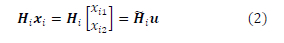
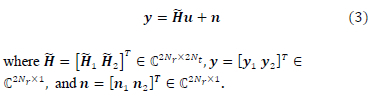
Wireless channel matrix Hi EC^NrX2Nt is the modified wireless channel matrix, for timeslot i, that includes the Golden code super symbol linear combination constants based on the equivalence relations in (2). The received signal vectors in (1), over timeslot i, are combined using the methodology as shown in [15] to produce (3)

To decode the transmitted M-QAM symbols SD-SDS is used based on the system model presented in (3). QR factorization is first performed on the modified wireless channel matrix H such that we get (4)

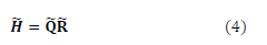
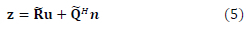
The matrix Q EC^2NrX2Nr is a unitary matrix and matrix R = [R₁ R₂]^T EC^2NrX2Nt has an upper triangular matrix R_x E C^2Nt^x2Nt and also a zero matrix R₂ EE.^(2Nr-^2Nt:^)x2Nt. The vector z = Q^Hy EC^2NrXl is the modified received signal vector over 2-timeslots, which is given by (5)

The low complexity SD-SDS detection algorithm proposed in [15] is summarized as follows:

SD-SDS Algorithm:

Step 1: Determine the complex M-QAM symbol estimates using QR-decomposition. Estimate x_q where q E [1: 4].

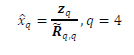
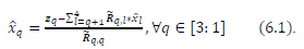
where z_q is the q^th scalar element stored in vector z and R_qq is the scalar element stored in the 17^th row and 17^th column of the matrix R.

Step 2: Determine the Fixed SD-SDS initial radius

From [15], the initial radius is calculated based on [20, Eqn (28)].

Step 3: Create the sorted detection subsets

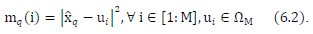
Using the M-QAM symbol estimates found in (6.1), sort in ascending order the M-QAM signal constellation for each estimated symbol based on the Euclidean distance squared metric in (6.2). The sorting is done in such a way that the complex symbols in the signal constellation are ordered in ascending order based on which complex symbol is closest to the estimated M-QAM symbols

This implies that for each estimated M-QAM symbol, x_q, we need to find the associated M-QAM symbols, sorted in ascending order, of the M - 1 nearest neighbors from the M-QAM signal constellation. Furthermore, depending on the average SNR, a subset of the sorted M-QAM constellation symbol order is used for detection. The subset lengths (L) are stated in [15, Table 2]. The sorting and L-dimensional subset determination is shown in (6.3):

 

 

 

 

 

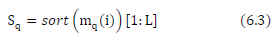
where S_q,V(7 6 [1:4], are the L-dimensional sorted subsets used in the detection of the optimal estimated transmitted symbols x₁,x₂,x₃, and x₄.

Step 4: Perform SD-SDS to determine candidates in hypersphere

The lattice point candidates which are being searched for, using SD-SDS, must lie inside the hypersphere stated in (6.4) as per [15]

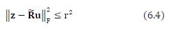
where r is the fixed initial radius determined in Step 2. The SDS found in Step 3 are used to search for these lattice point candidates that satisfy (6.4).

 

IV. GOLDEN CODE 2-TIMESLOT SD-SDS INITIAL RADIUS

This section presents two approaches to calculate the SD-SDS initial radius for the 2-timeslot Golden code scheme. The first approach is the fixed initial radius that we will derive for the 2-timeslot scheme and show that the single timeslot initial radius formula used by [15] is valid but was not justified in their paper. The fixed initial radius approach brings the disadvantage of finding many lattice points meeting the constraint stated in (6.4), under low average SNR conditions, in situations where the instantaneous SNR is high. This creates high detection complexity at lower average SNR values as it will be shown that at low average SNR values, the initial radius is large. The second approach involves a deep learning model that is used to predict the initial radius. The difference here is that the predicted initial radius depends on the instantaneous channel conditions instead of the average channel conditions. This means for each channel use, the initial radius is adapted to select a minimal number of lattice point candidates and thus reduce complexity. This idea is borrowed from [16] with a modification of the algorithm. Section IV-A presents the fixed initial radius derivation justifying using a single timeslot initial radius calculation for a 2-timeslot scheme. Section IV-B presents the adaptive initial radius deep neural network model.

A. DERIVATION OF FIXED INITIAL RADIUS

This section presents the proof of the 2-timeslot Golden code SD-SDS fixed initial radius as dependent only on a single timeslot. Hence, the traditional single timeslot initial radius formulae can be used for the 2-timeslot SD-SDS. We simplify (6.4) using (5) to get the expression

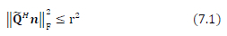
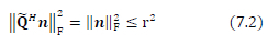
But we know that Q is unitary which implies that Q Q - l2N_r - QQ^H where 7_2Nr eR^2NrX2Nr is an identity matrix. This also implies that the matrix Q^H is unitary. We know from linear algebra that a vector's Frobenius norm is invariant to the multiplication with a unitary matrix [25]. Therefore, we can simplify (7.1) to get (7.2)

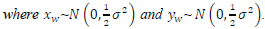
Lemma 1: We know that the noise vectors n₁ and n₂ are N_r-dimensional and that each entry n_w is distributed based on the zero-mean complex Gaussian distribution CN(0,a²). We also know that each noise vector entry is defined as a complex number as show in (7.3)

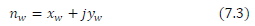
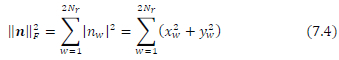
. Taking the square of a Frobenius norm of a 2N_r -dimensional noise vector n yields the following in (7.4)

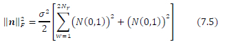
Using the laws of linear combination of variances, we have (7.4) being re-written as (7.5)

But since our sphere decoding algorithm will only search for lattice points using the upper half of the 2N_r-dimensional received signal vector z, as per [15], the lower half only contains noise and no signal. Therefore, we only need to consider the upper half of the 2N_r -dimensional noise vector n. This means (7.6) becomes the relevant expression for our use case

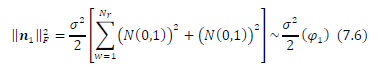
From Lemma 1 it follows that ||n||²_Fis a random variable where (φ₁)~X²(2N_r) is x² distributed with 2N_r degrees of freedom. The random variable (φ₁)~r(shape = N_r, scale = 2) is also Gamma distributed with a shape of N_r and a scale of 2. In order to get the sphere decoder initial radius r we need to set (φ₁)< r², thus (φ₁)< . Therefore, we can set the probability that the Gamma distributed random variable φ₁ is always less than or equal to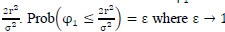. In our case, we set ε = 0.995 for 16-QAM and 0.9999 for 64-QAM. This implies that Prob(φ <P_E) =£. So, we will find the 99.5% or 99.99% percentile value P_E for the Gamma distributed random variable φ₁. Then we derive the sphere decoder initial radius as:

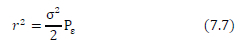
But we know that . This derivation proves that eventhough Golden code is a 2-timeslot scheme, the fixed initial radius is only dependent on the first timeslot, as shown in (7.6). Hence the single timeslot initial radius formulas in literature may be applied in SD-SDS. It also proves that as the average SNR Y -> 0 dB then r² approaches a large value based on (7.7) since

B. ADAPTIVE INITIAL RADIUS

In this section we present a Golden Code 2-timeslot deep neural network (DNN) SD-SDS radius predictor by extending the single timeslot DNN SD radius predictor found in [16] to a 2-timeslot DNN. Our DNN SD-SDS radius predictor has inputs from both timeslots 1 and 2. The inputs are stacked into a vector of size 2N_r(iV_t + 1) as shown in (8)

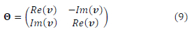
The entries dimensional received signal row vectors from (1). The entries vec(h_i)^r, i ε [1: 2] are the vectorized channel matrix entries from (1). We then convert the complex-valued vector in (8) into a real-valued matrix 0 εR^2x4Nr(Nt+1) as shown in (9) from [26]

Since this is supervised learning, the offline training of the DNN is done with an output label in the form of the distance squared of the lattice point closest to the upper half of the received signal vector z. This translates to the closest lattice radius to the upper half of the received signal vector z. The radius is found from the SD-SDS assisted ML detector output distances for each possible combination of the 4 M-QAM symbols. The radius or distance squared for the lattice point with the smallest distance from the received signal vector is computed in (10) [16]

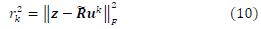
where u^k is the k^th smallest radius lattice point found inside the hyper-sphere of radius r². The initial radius used for the SD-SDS is based on the derived fixed initial radius in (7.7) of this paper. The radii or distances for the candidate lattice points are sorted in ascending order as follows: , where K is a large number of candidates, especially at lower SNR as shown in (7.7). The smallest radius is loaded into a 1-dimensional vector r=[r₁²] and is used as the output label data for the input training data generated using (8) and (9).

We only select one radius as the output label because during training we realized that because SD-SDS is a lower complexity detection algorithm relative to SD, sometimes there is only one lattice point that lies within the hypersphere radius. The number of lattice points found inside the hypersphere fluctuates from one-to-many candidates. To collect as many training data points as possible, we select all possible number of lattice points from 1 point to the largest possible number. The input and output training data are normalized or scaled into the interval [0,1]. The scaling for the input feature data X is carried out using the formula X = per input feature. X_min is the smallest feature value over all training SNR values and X_max is the highest feature value over all training SNR values.

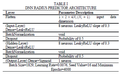
The DNN in Table I is trained from 30dB to 2dB SNR range from the highest SNR value to the lowest. The output label data Y is scaled using the formula Y = 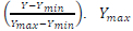is the maximum radius value of the lattice points and Y_min is the minimum radius value over the whole SNR training range. From experimentation, we observe that the output linear activation function used in [16] yields negative radiuses. This motivates us to use a bounded activation function such as the Sigmoid activation function since the radius values cannot be negative and further to that, the radius values do get quite large at low average SNR which negatively affects the training performance of the DNN. The training data is then used to train the neural network in Table I to minimize the mean squared error loss function using the ADAM optimizer [27].

We notice from observation that the DNN architecture is sensitive to the input Matrix or Vector shape or size. This implies that the DNN architecture in Table I is valid for a 2x4 MIMO configuration since our training is based on this MIMO configuration. The baseband modulation schemes used in training the DNN in Table I are the 4-QAM, 8-QAM, 16-QAM and 64-QAM data symbols. For any other MIMO configuration and modulation schemes, a new architecture will need to be selected and trained. During operation, the DNN in Table I will be used as an adaptive initial radius predictor based on the normalized instantaneous received signal vectors and wireless channel matrices from timeslot 1 and 2 as per (8) and (9). The predicted output radius from the DNN in Table I is de-normalized back to the initial radius's original scale. The formula used for de-normalizing the predicted radius is r² = (Y_max - Y_min) x ^r2p_red + Y_min where r²_pred is the normalized predicted radius in the range [0,1] and r² is the de-normalized predicted radius.

 

V. GOLDEN CODE SD-SDS DEEP LEARNING ALGORITHMS

This section is dedicated to exhibiting the algorithms developed to lower complexity in Golden code SD-SDS detection. Section V-A ventilates the SD-SDS-Radius-DNN algorithm that aims to lower the detection complexity of SD-SDS at mid-to-low SNR. This algorithm uses the adaptive initial radius DNN predictor, in Table I, to predict the SD-SDS initial radius based on the instantaneous channel conditions as per [16]. Section V-B exhibits the novel SD-SDS-DNN algorithm that executes the SD-SDS-Radius-DNN algorithm under unfavorable instantaneous channel or noise conditions and the QR decomposition suboptimal detector is preferred in favorable instantaneous channel and noise conditions. The SD-SDS-DNN algorithm lowers the detection complexity of the SD-SDS at low SNR by preferably running the low complexity QR decomposition sub-optimal detector under favorable instantaneous channel and noise conditions.

A. SD-SDS-Radius-DNN ALGORITHM

SD-SDS-Radius-DNN algorithm:

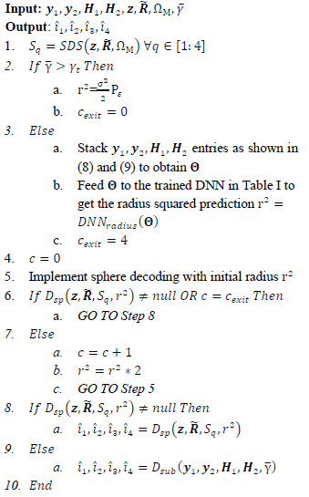
where D_sp(.) is the SD algorithm as implemented in [15], D_sub (.) is the sub-optimal detector of M-QAM symbols when the SD algorithm finds no lattice points candidates. y_t is the average SNR threshold below which the adaptive initial radius DNN algorithm is activated. y_t is defined as 11 dB for 16-QAM and 19 dB for 64-QAM. The SD-SDS algorithm has low detection complexity at high SNR and higher detection complexity at lower SNR values as stated in [15]. The values 11 dB and 19 dB are found via experimentation after observing that the SD-SDS-Radius-DNN algorithm effectively reduces complexity below a specific average SNR threshold. The 16-QAM case was found to be effective from 11 dB downwards and for 64-QAM it was found to lower detection complexity from 19 dB downwards. In this paper, we are targeting the high detection complexity at lower SNR values for SD-SDS. Therefore, the thresholds basically determine when the adaptive initial radius predictor must take effect and reduce detection complexity. SDS(. ) is the sorted detection subset algorithm as detailed in Step 3 of Section III. i₁,i₂,i₃,i₄ are the decoded M-QAM symbol indices.

The SD-SDS-Radius-DNN algorithm is a modified version of the algorithm in [16]. The SD-SDS-Radius-DNN algorithm is modified to suit the SD-SDS context of having only 1 predicted radius output. This means that if no lattice point candidates are found within the predicted radius of the hypersphere, we need a way to increase the hypersphere radius and perform the sphere-decoding again. We are inspired by the idea in [17] of iteratively dividing the hypersphere radius by 2 and feeding the updated radius to a DNN to predict the number of lattice points inside a hypersphere. In our case, we do the opposite; if we do not find lattice point candidates inside the hypersphere, we increase the radius by multiplying it by a factor of 2 until we reach a pre-determined iteration limit of 5 set as c_exit = 4. The c_exit limit is set via a heuristic method by considering that a high iteration limit leads to higher detection complexity or latency. A lower iteration limit leads to sub-optimal BER performance as the sub-optimal detector will be relied on more often. The algorithm also has the DNN prediction of the initial radius only done below a certain average SNR threshold since SD-SDS has a high detection complexity at lower SNR values whilst at higher SNR values, it has low detection complexity. When the SD-SDS-Radius-DNN algorithm fails to find lattice point candidates inside the hypersphere of a pre-determined radius, the LMMSE estimator x_i = (H^H_i H_i + σ²/_Nt) H^H_iy_i i ε [1:2] from [16] is used as a sub-optimal detector for Golden code symbol estimates. The vector x_i is the sub-optimally estimated transmitted Golden code symbol vector for timeslot i. The 4 square M-QAM symbols conveyed by these estimated Golden code symbols are then found using expression (11.1) to (11.2) which are adapted from [14]

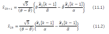
where k ε [1: 2].

Therefore, we can search for the symbol indices that minimize the following Euclidean distances squared based on (12) for each estimated square M-QAM symbol.

B. SD-SDS-DNNNOVEL ALGORITHM

The SD-SDS-DNN algorithm uses the instantaneous channel conditions and received signal vectors to predict, using a DNN, whether the sub-optimal QR decomposition M-QAM symbol estimates, found in Step 1 of the SD-SDS algorithm in Section III, are good enough to be used as the actual transmitted symbols without performing the SD-SDS-Radius-DNN based search. The output of the DNN is a probability value in the range [0,1] that is used to determine whether the channel conditions and instantaneous noise values in the received signal vectors are good enough to directly output the transmitted M-QAM symbols from the QR decomposition sub-optimal detector. If the probability is greater than a specific threshold, then the QR decomposition sub-optimal detector output is taken as the transmitted symbols. If it is less, then the more complex SD-SDS-Radius-DNN based search is performed.

Let us define the proposed DNN which predicts the channel condition state probability based on the instantaneous channel conditions and noise statistics. We define the DNN as

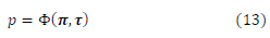
where p ε [0,1] is the probability that the channel conditions are sufficient to use the QR decomposition sub-optimal detector estimated M-QAM symbols as the transmitted M-QAM symbols. The function Φ(-) is the DNN channel condition state predictor which takes the input vector n = [z^R,z¹,r^R₁ ,r^I₁] ε R²⁸ which is a combination of the modified received signal vector in (5) and the upper triangular matrix R₁The entries of the vector n are real valued as the DNN function approximator can only take real numbers. We define z^R 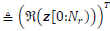. 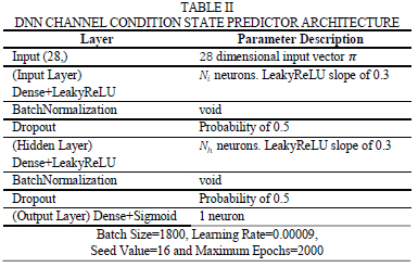The notation z[0:N_r) means that we take the first N_r elements of the vector z since the last N_r elements are just noise without any signal. With regards to the upper triangular matrix we only take the non-zero real valued elements of the matrix entries. The DNN input vector n is a 28-dimensional vector because the DNN architecture in Table II is trained for a fixed MIMO configuration of N_t = 2 and N_r = 4. For any other MIMO configuration the DNN architecture in Table II will change and will need to be re-trained. The vector T is a vector of all hyperparameters that need to be tuned during the training phase of the DNN.

The DNN function approximator Φ(-) has an architecture shown in Table II.

where N_t is the number of input layer neurons and N_h is the number of hidden layer neurons. For the architecture in Table II to be useful, we need to train the DNN architecture with appropriate training samples and test the DNN before deploying it. The next section attends to this.

i. TRAINING AND TESTING PHASE

The objective of this phase is to tune the weights and biases of the DNN function which are found in the vector . The DNN function in Table II is trained using approximately 10 000 samples of data over an average SNR range of [0,21] dB for 16-QAM modulation and [10,28] dB for 64-QAM modulation. The DNN is trained from the highest average SNR value to the lowest average SNR value. The way the training data is collected is based on the following pseudocode:

Training Pseudocode:

###Start Comment ###

### X is the input sample array and Y is the output label sample array

###end comment###

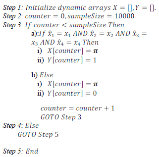
The idea is that when the instantaneous channel conditions are very good, then the condition in Step 3 a) can be easily met and the training output label value is set to 1. When the instantaneous channel conditions are not favorable then the condition in 3a) is most likely not met and the output label value is set to 0. The reasoning is that when the instantaneous fading channel conditions are good and instantaneous noise power is low, the QR decomposition M-QAM symbol estimates x_q,Vq ε [1,4] will be a good enough estimate for the actual transmitted M-QAM symbols x_q,Vq ε [1,4]. After collecting the input and output training data, since this is a supervised learning problem, we trained the DNN and realized that the validation accuracy of the DNN under test conditions was in excess of 99% for high and low SNR values. In the mid-SNR range, the validation accuracy went as low as 36%.

Upon inspection of the training data, we realized that the collected training samples were skewed. The output label distribution was not evenly distributed between the 0 state and 1 state for both high and low average SNR values. Fig. 1 and 2 illuminate the distribution of the output label states for 16-QAM and 64-QAM, respectively.

 

 

 

 

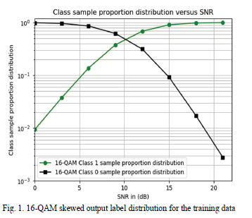
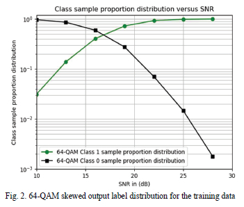
This explained why the DNN was underperforming in the mid-SNR range whilst performing in the high and low SNR region. This is because the DNN became lazy to learn and decided to memorize the output state and retain the output predicted state on one state depending on whether it is the low SNR or high SNR region. In the high SNR region, the DNN will constantly output a predicted state of 1 because over 99% of the output labels have values of 1. The objective is to maximize the validation accuracy and the DNN can achieve this by just outputting a predicted state of 1 for the high SNR case. The same logic applies for the low SNR case.

To force the DNN to learn during training, we decided to perform over-sampling of the minority state/class and under-sampling of the majority state/class for the full SNR range. The over-sampling is performed using the synthetic minority over-sampling technique (SMOTE) [29] and the under-sampling is performed using randomized under-sampling of the majority class [29]. The SMOTE works by randomly selecting a minority class/state feature sample in the training data and then using the if-nearest neighbor (KNN) algorithm to select the K nearest neighbors to that selected feature sample. It then randomly selects one nearest neighbor from the selected K neighbors and randomly creates a new synthetic feature sample point on the line joining the chosen nearest neighbor feature sample and the originally selected feature sample on the R²⁸ dimensional cartesian plane. The process is repeated until a desired sample size of the minority class is achieved. The under-sampling is performed by randomly selecting a feature sample in the majority class/state and then deleting it from the training samples. This is repeated until a desired ratio between the majority class and minority class is achieved. In our case, we performed this until the majority class was approximately 60% of the training sample size and the minority class 40% for the full average SNR range for both 16-QAM and 64-QAM training data.

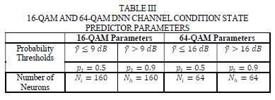
We then went ahead to train the DNN architecture in Table II using this modified training data with 25% of the training samples being used for testing purposes and 75% for training. The input feature training data in array X was scaled into the range [0,1] using the methodology explained in Section IV-B. The loss function selected for the optimization of the DNN hyperparameters was the binary cross entropy loss function with the validation accuracy used as the metric to measure performance. The ADAM optimizer [27] was used to perform the optimization of the DNN weights and biases in the vector T by comparing the output of the DNN to the target values in array Y. During the testing phase, the DNN is fed multiple test vectors n from the test samples and the output of the DNN predicts a probability value in the range [0,1]. Table III shows the probability thresholds p_t and number of neurons used in the architecture for the case of 16-QAM and 64-QAM. The probability thresholds are used to determine the channel condition state. If the predicted probability exceeds a given probability threshold p_t, then the channel condition state is 1. If the predicted probability is less than or equal to the probability threshold p_t, then the channel condition state is 0.

 

 

ii.SD-SDS-DNN ALGORITHM EXPLAINED

The DNN function approximator in Table II is used to predict when the QR decomposition M-QAM symbol estimates can be used as appropriate estimates for the transmitted M-QAM symbols. The SD-SDS-DNN algorithm combines this DNN function approximator in Table II, the SD-SDS algorithm developed in [15] and the SD-SDS-Radius-DNN algorithm. The SD-SDS-DNN algorithm is presented as follows:

SD-SDS-DNN algorithm:

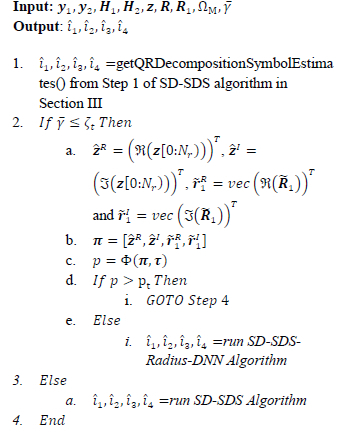
From the SD-SDS-DNN algorithm we can see that when the average SNR y exceeds the threshold £_t the SD-SDS algorithm from [15] is executed. This is because at high SNR values the detection complexity of the SD-SDS algorithm is very low. The objective of this paper is to reduce the detection complexity of the SD-SDS algorithm at low SNR values. At lower SNR values, y < ζ_t the SD-SDS-DNN algorithm executes the DNN channel predictor in Table II that is used to select between the very low complexity sub-optimal QR decomposition detector and the execution of the low complexity near-optimal SD-SDS-Radius-DNN detector. The average SNR thresholds for 16-QAM and 64-QAM modulation are ζ'_t = 6 dB and ζ_t = 19 dB, respectively. The thresholds p_t and ζ_t are found using a heuristic method.

From the SD-SDS-DNN algorithm we observe that when the predicted probability from the DNN exceeds the probability threshold p_t, as shown in Table III, then the SD-SDS-Radius-DNN algorithm does not get executed at all. The estimated transmitted M-QAM symbols come directly from the very low complexity QR decomposition sub-optimal detector. If the predicted probability is less than or equal to the probability threshold pt, then the SD-SDS-Radius-DNN algorithm gets executed as the QR decomposition sub-optimal detector output is deemed unreliable by the DNN predictor.

 

VI. COMPLEXITY ANALYSIS OF PROPOSED ALGORITHMS

In this section, we will deal with the detection complexity analysis of the three different Golden code detection algorithms discussed here and in literature. The detection complexity is defined in various ways using different metrics. We will extend the detection complexity metric of evaluating complexity using the number of complex-valued operations [30] performed by a detection algorithm. Since some of the algorithms rely on deep neural networks, which only process real values, we will only consider complexity analysis of real-valued floating-point operations (FLOPS) [14]. The real-valued binary operators of interest are the multiplication, addition, subtraction, and division as per [14]. We also neglect the sub-optimal detector's detection complexity since it is only executed 0.5% of the time for 16-QAM and 0.01% for 64-QAM Monte-Carlo simulations. Its contribution to the average detection complexity is marginal. The DNN complexity analysis of the offline training and data collection is ignored because offline training is done only once [16]. We are only performing the DNN complexity analysis for the online decoding process.

In [16], the detection complexity metric used is the decoding time and order of execution, whilst [17] uses the number of lattice points inside the hypersphere and the average processing time for the decoding process. Our complexity analysis is based on the number of floating-point operations; hence we cannot use any of the complexity results in [16] and [17] as a benchmark against our detection complexity. Our complexity analysis is relative between the Alamouti linear ML, Golden code SD, SD-SDS, and SD-SDS-DNN algorithms for the 2x4 MIMO configuration. In [15], they use the number of Euclidean distance calculations as the metric for the complexity analysis of SD-SDS. This again is different from our metric and makes the results in [15] not comparable to ours.

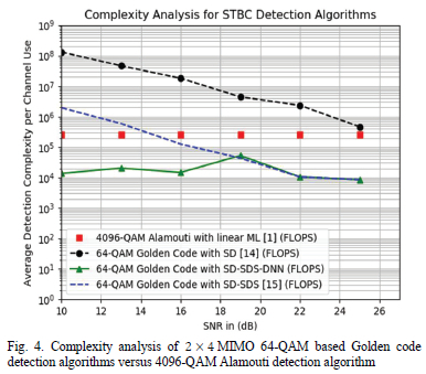
The detection complexity of the three Golden code detection algorithms, SD, SD-SDS, and SD-SDS-DNN is determined using simulations. The results are exhibited in Fig. 3 and 4. The detection complexity of the Alamouti STBC linear ML detector is also exhibited in Fig. 3 and 4. The Golden code detection algorithms are evaluated in a fast-fading wireless environment; however, it is interesting to see its performance against the Alamouti STBC in a block-fading wireless channel. The reason for this is that we aim to achieve lower detection complexity relative to the low complexity Alamouti linear ML detector which performs optimally in block-fading wireless channels [4]. The Alamouti STBC scheme's modulation order is selected as 256-QAM so that the spectral efficiency of the scheme matches that of the 16-QAM Golden code STBC scheme which is 8 bits/s/Hz. The Alamouti STBC scheme's modulation order is also selected as 4096-QAM so that the spectral efficiency of the scheme matches that of the 64-QAM Golden code STBC scheme which is 12 bits/s/Hz. This makes the comparison fair between the two schemes as we want to see the detection complexity of the two competing STBC schemes for the same achieved spectral efficiency.

 

 

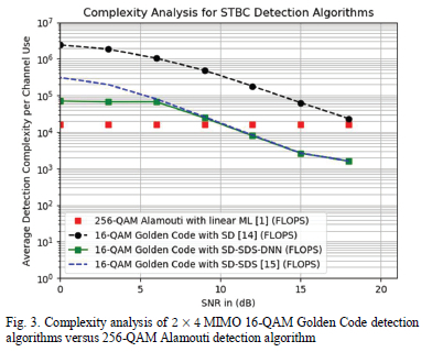
As can be seen in Fig. 3, the proposed SD-SDS-DNN algorithm outperforms the SD-SDS algorithm developed in [15] at low SNR. We observe that the detection complexity is identical between 6 dB and 18 dB because the SD-SDS algorithm is executed when the average SNR exceeds the 6 dB threshold as per the SD-SDS-DNN algorithm. This is because the SD-SDS algorithm exhibits low detection complexity at high SNR values. The low complexity SD-SDS-Radius-DNN algorithm, that runs within the SD-SDS-DNN algorithm, only has an opportunity to be executed when the average SNR is equal to or less than 6 dB. From 6 dB and below, the SD-SDS-DNN algorithm exhibits lower detection complexity relative to the SD-SDS algorithm. This is because the low complexity QR decomposition detector or the SD-SDS-Radius-DNN algorithm are being selected as M-QAM symbol detectors depending on instantaneous channel conditions and noise. In Table IV, we get the insight of the percentage distribution of how many times the predicted transmitted symbols were determined by the suboptimal QR decomposition method, SD-SDS decoder or the SD-SDS-Radius-DNN decoder, for 16-QAM modulation.

 

 

 

 

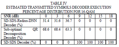
It is clear from Table IV that the SD-SDS algorithm is solely used at high SNR for its low detection complexity. For 6 dB SNR and below, the QR decomposition sub-optimal detector is used in most cases to predict the transmitted symbols compared to the SD-SDS-Radius-DNN decoder. Hence the 75% reduction in detection complexity at low SNR relative to the SD-SDS decoder, as shown in Fig. 3, is due to the mix in the low complexity detection of the QR decomposition sub-optimal detector and the SD-SDS-Radius-DNN decoder.

In Fig. 3, we also notice that the SD-SDS-DNN algorithm has a detection complexity that is 4 times greater than that of the Alamouti STBC linear ML detector, at low SNR. At high SNR, the SD-SDS-DNN algorithm has 90% lower detection complexity relative to the Alamouti STBC linear ML detector. This shows that Golden code has a future in practical MIMO applications since the detection complexity has been reduced such that it is comparable to that of the Alamouti linear ML detector. With regards to the traditional SD algorithm, it is shown in Fig. 3 that its detection complexity is the highest amongst the STBC detection algorithms discussed in this paper.

In Fig. 4, the proposed SD-SDS-DNN algorithm outperforms the SD-SDS algorithm developed in [15] at low SNR. We observe that the complexity is identical between 19 dB and 25 dB because the SD-SDS algorithm is executed as a detector of choice above the 19 dB average SNR threshold as per the SD-SDS-DNN algorithm. Below 19 dB, the instantaneous channel and noise conditions are used to select between the very low complexity sub-optimal QR decomposition detector and the low complexity SD-SDS-Radius-DNN detector. When the instantaneous channel and noise conditions are very good, the DNN channel condition predictor in Table II selects the very low complexity QR decomposition detector as a detector of choice. When the instantaneous channel conditions are unfavorable, the more complex SD-SDS-Radius-DNN detector is executable as it produces reliable symbol estimates even when the instantaneous channel and noise conditions are unfavorable.

In Table V, we exhibit the percentage distribution of how many times the predicted transmitted symbols were determined by the sub-optimal QR decomposition method, SD-SDS decoder or the SD-SDS-Radius-DNN decoder, for 64-QAM modulation.

 

 

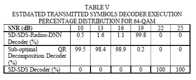
It is clear from Table V that the SD-SDS algorithm is solely used at high SNR for its low detection complexity. For 16 dB SNR and below, the QR decomposition sub-optimal detector is used at least 98% of the time to predict the transmitted symbols compared to the less than 2% utilization of the SD-SDS-Radius-DNN decoder. Hence the 99% lower detection complexity, at low SNR, relative to the SD-SDS decoder, as shown in Fig. 4, is largely due to the low complexity detection of the QR decomposition sub-optimal detector.

From Fig. 4, we observe that the proposed SD-SDS-DNN algorithm outperforms the Alamouti linear ML detector by exhibiting a detection complexity that is 90% lower for the greater part of the SNR range. We also observe that the traditional SD algorithm is the most computationally complex detection algorithm relative to the STBC detection algorithms discussed in this paper.

 

VII. simulation results and discussions

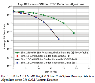
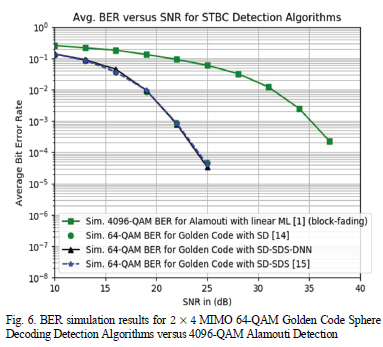
The Monte-Carlo wireless simulation environment was setup as a 2x4 MIMO, where N_t = 2 and N_r = 4, with a wireless channel with Rayleigh frequency-flat fast fading in which the channel gain changes per transmission timeslot. The wireless channel transmit-and-receive antennas are sufficiently spaced such that the wireless channels are de-correlated. The information symbol modulation order used in the simulation was 16-QAM and 64-QAM. The average power constraint for the 16-QAM and 64-QAM symbols was set to 1. The SD fixed initial radius probability was set to ε=0.995 for 16-QAM and ε=0.9999 for 64-QAM. The Monte-Carlo simulation determined the BER performance of the three detection algorithms SD, SD-SDS and SD-SDS-DNN for 16-QAM and 64-QAM. We also simulated the BER performance of the 256-QAM Alamouti STBC scheme within a block-fading wireless channel. We chose the 256-QAM constellation for the Alamouti scheme so that the spectral efficiency of the Alamouti STBC and 16-QAM Golden code schemes were identical. This allowed us to compare the BER performance of Alamouti against that of the Golden code STBC. The 64-QAM Golden code STBC produced the same spectral efficiency as the 4096-QAM Alamouti scheme.

If we look at Fig. 5, we see that the proposed SD-SDS-DNN algorithm achieves the same BER performance as SD and SD-SDS algorithms from literature for 16-QAM. This means that the detection algorithm achieves the objective of lowering the detection complexity of SD-SDS, at low SNR, without compromising the BER performance. The Golden code STBC scheme has an 8 dB signal power gain over the Alamouti STBC scheme at a BER of 10^-3 for a spectral efficiency of 8 bits/s/Hz. This implies that the Golden code STBC can achieve the same spectral efficiency as the Alamouti STBC scheme but at a much higher link reliability and comparable detection complexity with the linear ML detector as shown in Fig. 3.

 

 

In Fig. 6, we see that the proposed SD-SDS-DNN algorithm achieves the same BER performance as SD and SD-SDS algorithms from literature for 64-QAM. This means that the detection algorithm achieves the objective of lowering the detection complexity of SD-SDS, at low SNR, without compromising the BER performance. The Golden code STBC scheme has a 13 dB signal power gain over the Alamouti STBC scheme at a BER of 10^-3 for a spectral efficiency of 12 bits/s/Hz. This implies that the Golden code STBC can achieve the same spectral efficiency as the Alamouti STBC scheme but at a much higher link reliability and 90% lower detection complexity relative to the linear ML detector as shown in Fig. 4.

 

 

VIII. conclusion and future work

The SD-SDS-DNN algorithm was developed in our research to lower detection complexity of SD-SDS, at low SNR, whilst maintaining the BER performance. The SD-SDS-DNN algorithm is shown to reduce the detection complexity relative to SD-SDS by at least 75%, at low SNR, for 16-QAM. For 64-QAM, the detection complexity of the SD-SDS-DNN algorithm is at least 99% lower than that of SD-SDS at low SNR. This is all achieved whilst maintaining the BER performance close to that of SD-SDS and SD from literature. The SD-SDS-DNN algorithm lowers the detection complexity of Golden code to the point that it approaches the detection complexity of the Alamouti STBC linear ML detector for a spectral efficiency of 8 bits/s/Hz. For a spectral efficiency of 12 bits/s/Hz, the SD-SDS-DNN detection complexity is 90% lower than the Alamouti linear ML detector detection complexity.

In future research, the SD-SDS-DNN algorithm DNN channel condition predictor may be replaced with a low computational complexity random forest ensemble decision tree which may further reduce detection computational complexity in terms of number of FLOPS. Determination of the order of execution of the DNN detection algorithms in terms of inference time will be of value from a detection latency point of view.

 

References

[1]. S. M. Alamouti, "A simple transmit diversity technique for wireless communications," IEEE Journ. Sel. Areas Commun., vol. 16, no. 8, pp.1451-1458, 1998.         [ Links ]

[2]. H. Xu, K. Govindasamy, and N. Pillay, "Uncoded space-time labelling diversity," IEEE Commun. Lett., vol. 20, no. 8, pp. 1511-1514, 2016.         [ Links ]

[3]. J. Belfiore, G. Rekaya and E. Viterbo, "The golden code: a 2 x 2 full-rate space-time code with non-vanishing determinants," International Symposium on Information Theory, ISIT 2004. Proceedings., Chicago, IL, 2004, pp. 310-310, 2004.

[4]. A. Vielmon, Ye Li and J. R. Barry, "Performance of Alamouti transmit diversity over time-varying Rayleigh-fading channels," IEEE Trans, on Wireless Commun., vol. 3, no. 5, pp. 1369-1373,2004.         [ Links ]

[5]. M. O. Sinnokrot and J. R. Barry, "Fast maximum-likelihood decoding of the Golden code," IEEE Trans. Wireless Commun., vol. 9, no. l,pp. 26-31,2010.         [ Links ]

[6]. N. Sharma, "Space Time Block Code for Next Generation Multi-user MIMO System," 9th International Conference on Future Networks and Communications, Procedia Computer Science, pp. 172-179,2014.

[7] F. Riera-Palou and G. Femenias, "Improving STBC Performance in IEEE 802.1 In Using Group-Orthogonal Frequency Diversity," IEEE Wireless Communications and Networking Conference, Las Vegas, NV, pp. 193-198, 2008.

[8]. "IEEE Standard for Information technology- Telecommunications and information exchange between systems - Local and metropolitan area networks-Specific requirements -Part 11: Wireless LAN Medium Access Control (MAC) and Physical Layer (PHY) Specifications Amendment 2: Sub 1 GHz License Exempt Operation," in IEEE Std 802.11ah-2016 (Amendment to IEEE Std 802.11-2016, as amended by IEEE Std 802.11ai-2016), pp.1-594, 2017.

[9]. M. O. Sinnokrot and J. R. Barry, "Fast maximum-likelihood decoding of the Golden code", IEEE Trans. Wireless Commun., vol. 9, no. 1, pp. 26-31, 2010.         [ Links ]

[10]. S. Kahraman and M. E. Celebi, "Dimensionality reduced decoding for the golden code with the worst-case complexity of O(m¹⁵) for low range of SNR," IEEE Wireless Communications and Networking Conference (WCNC), 2012, pp. 246-250. [11]. S. Sirinaunpiboon, A. R. Calderbank, and S. D. Howard, "Fast essentially maximum likelihood decoding of the Golden code," IEEE Trans. Inf. Theory, vol. 57, no. 6, pp. 3537-3541, 2011.         [ Links ]

[12]. L. Zhang, B. Li, T. Yuan, X. Zhang, and D. Yang, "Golden code with low complexity sphere decoder," in Proc. 18th Int. Symp. Pers. Indoor Mobile Radio Commun., pp. 1-5, 2007.

[13]. J. Jaldén and B. Ottersten, "On the complexity of sphere decoding in digital communications", IEEE Trans. Signal Process., vol. 53, no. 4, pp. 1474-1484, 2005.         [ Links ]

[14]. H. Xu and N. Pillay, "Reduced complexity detection schemes for Golden code systems," IEEE Access, vol. 7, pp. 139140-139149, 2019.         [ Links ]

[15]. H. Xu and N. Pillay, "Multiple complex symbol Golden Code," IEEE Access, vol. 8, pp. 103576-103584, 2020.         [ Links ]

[16]. M. Mohammadkarimi, M. Mehrabi, M. Ardakani and Y. Jing, "Deep Learning-Based Sphere Decoding," IEEE Trans. on Wireless Commun., vol. 18, no. 9, pp. 4368-4378, 2019.         [ Links ]

[17]. A. Askri and G. R. Othman, "DNN assisted Sphere Decoder," 2019 IEEE Int. Symposium on Inf. Theory (ISIT), Paris, France, pp. 1172-1176, 2019.

[18]. N. T. Nguyen, K. Lee and H. Dai, "Application of Deep Learning to Sphere Decoding for Large MIMO Systems," in IEEE Transactions on Wireless Communications, DOI: 10.1109/TWC.2021.3076527.

[19]. D. Weon and K. Lee, "Learning-aided deep path prediction for sphere decoding in large MIMO systems," in IEEE Access, vol. 8, pp. 70870-70877, 2020        [ Links ]

[20]. B. M. Hochwald and S. ten Brink, "Achieving near-capacity on a multiple-antenna channel," IEEE Trans. on Commun., vol. 51, no. 3, pp. 389-399, 2003.         [ Links ]

[21]. J. Li and Z. Wang, "An improved initial radius selection scheme for sphere decoding in MIMO", 3rd Int. Conference on Advances in Electrical, Electronics, Information, Communication and Bio-Informatics (AEEICB17).

[22]. B. Hassibi and H. Vikalo, "On the sphere-decoding algorithm I. Expected complexity", IEEE Trans. on Signal Processing, vol. 53, no. 8, pp. 2806-2818, 2005.         [ Links ]

[23]. J. Jalden and B. Ottersten, "On the complexity of sphere decoding in digital communications," IEEE Trans. on Signal Processing, vol. 53, no. 4, pp. 1474-1484, 2005.         [ Links ]

[24]. F. Oggier, "On the optimality of the Golden code", in Proc. IEEE Inf. Theory Workshop, Punte del Este, Uruguay, pp. 468472, 2006.

[25]. O. A. Ivanova, Unitary Matrix, Encyclopedia of Mathematics, EMS Press, 1994.

[26]. N. Samuel, T. Diskin, A. Wiesel, "Learning to detect" IEEE Trans. on Signal Processing, vol. 67, no. 10, 2019.         [ Links ]

[27]. D. B. J. Kingma, "Adam, a method for stochastic optimization", 2014.

[28]. C. Candan, "Notes on Linear Minimum Mean Square Error Estimators", 2011.

[29] N. V. Chawla, K. W. Bowyer, L. O. Hall, W. P. Kegelmeyer, "SMOTE: Synthetic Minority Over-sampling Technique", Journal of Artificial Intelligence Research, vol. 16, 2002.         [ Links ]

[30]. R. Y. Mesleh, H. Haas, S. Sinanovic, C. W. Ahn, and S. Yun, "Spatial modulation", IEEE Trans. Veh. Technol., vol. 57, no. 4, pp. 2228-2241, 2008.         [ Links ]

 

 

 

Bhekisizwe Mthethwa received the BScEng Electronics degree from the University of KwaZulu-Natal in 2008 and the MScEng Electronics degree (Summa Cum Laude) in 2013 from the same institution. He has over 10 years industrial experience ranging from Mining consulting as a Control and Instrumentation Engineer to a senior system engineer within the Research and Development space. He has been involved in projects from designing and constructing furnaces, software application development and system engineering work. He is a registered Professional Engineer with the Engineering Council of South Africa (ECSA). Mr Mthethwa's research interests include Spatial Modulation, MIMO SpaceTime Block Coding schemes and the application of Deep Learning to the design of wireless systems. Mr. Mthethwa is currently pursuing his PhD degree under the guidance of Dr. H. Xu. Mr Mthethwa is also a reviewer for the Physical Communication Journal and IEEE Access.

 

 

Dr Hongjun Xu received the B.Sc. degree from the Guilin Institute of Electronic Technology (nowadays it is called Guilin University of Electronic Technology), Guilin, China, in 1984; the M.Sc. degree from the Institute of Telecontrol and Telemeasure, Shi Jian Zhuang, China, in 1989; and the Ph.D. degree from the Beijing University of Aeronautics and Astronautics, Beijing, China, in 1995. From 1997 to 2000, Dr. Xu was a Postdoctoral Fellow with the University of Natal (Nowadays it is called University of KwaZulu-Natal), Durban, South Africa, and Inha University, Incheon, Korea. Dr. Xu joined the University of Natal in 2002 as a lecturer. Dr. Xu has been a full Professor with the School of Engineering at the University of KwaZulu-Natal since 2011. Dr. Xu is also a rated scientist of the national research foundation in South Africa