Measurement-based load parameter modelling for technical and tariff studies of medium voltage feeders

 

 

Johannes L. Buys^I; Charles T. Gaunt^II

^IWorks at Eskom and was an MSc Electrical Engineering student at University of Cape Town, Rondebosch 7701, South Africa, (lolo.buys@gmail.com)
^IIEmeritus professor in the Department of Electrical Engineering, at University of Cape Town, Rondebosch 7701, South Africa (ct.gaunt@uct.ac.za).Fellow, SAIEE

 

 

---

ABSTRACT

Transformation in the South African power sector and new load patterns necessitated a review of load models used for financial, technical and tariff analysis. This pilot study took advantage of available data of customer measurements on medium Voltage (MV) feeders in Eskom's database. Load models with distinct profiles for typical days were developed for non-overlapping customer classes using a set of coherent parameters derived from MV chronological load profiles and the k-means algorithm. The results suggested that two profiles can be used to for summer and two profiles can be used for winter instead of using 365 hourly profiles for simulations. The results also reveal that load classification can be improved when the parameters are directed towards specific objectives, and also when the k-means algorithm is supervised using exogenous (external) parameters of loads. A comparison of the results to the economic activity class suggests that there are sub-clusters identifiable within the economic classes. The proposed process is practical, implementable with available data and suitable for various studies on MV networks.

Index Terms: Index Terms: Classification, clustering, load models, load profiles, medium voltage, measurement, tariffs, technical analysis.

---

 

 

I. Introduction

LOAD models are used to represent the energy usage patterns of customers in power systems studies [1], [2]. The proliferation of energy efficiency systems and distributed generation (DG) based on renewable energy changed the load patterns on many feeders and increased uncertainty in modelling distribution networks [3], [4]. Weather, location and economic factors also affect load profiles [5], [6].

Technical applications of load models for customers in distribution networks include the calculation of voltage drops [7], the technical losses in the distribution system [8], demand forecasting [9], and DG integration planning [10] [11].

In South Africa, load models inform customer classification and demand, which are essential inputs to Eskom's geographical based load forecasting (GLF) tool [12]. The GLF is characterized by three main components: load position forecast (location), active and apparent power (kW or kVA), the anticipated period, and load class.

Probabilistic load models are used in network design in South Africa, particularly in low voltage (LV) feeder voltage calculations and were pivotal in the development of the Herman-Beta (HB) transform [13], [14]. The extended HB transform in medium voltage (MV) feeders [15] accommodates loads and DG with non-unity power factor, although few models of MV loads are available.

Worldwide, the role of load models in tariff analysis, forecasting and design is recognized [3], [9], [11], [16]. Tariffs also affect load profiles, network operations and planning [3],[17]. The drivers of load models for tariff analysis and design include load demand representation, cost of service and tariff objectives [18] [19].

Load models are part of the cost of supply models used in most utilities to provide energy forecasts per customer classes, and for setting time of use (TOU) intervals for TOU tariffs [16]. However often these load models are not formalized.

The connection of DG to the distribution systems has economic implications. The aspects of the distribution economics likely to be impacted by DG connections include the initial network investments, network upgrades, distribution operation and maintenance (O&M) costs, installation of voltage control schemes and protection devices, and changes in the network planning environment [20]. Cost-reflective models are needed to reduce consumers cross-subsidizing prosumers [20]. Cross-subsidization is unavoidable though, as it is inherent in aggregated distribution tariffs, and the use of volumetric tariffs to recover most of the costs from customers [16].

TOU tariffs, with generation standby charges and fixed charges, remove some unintended tariffs cross-subsidies. Fell et al [21] suggested that DG technologies such as combined heat and power (CHP), and renewables with stationary or electric vehicle (EV) storage, can be effective for peak shaving and providing energy when needed, and managing congestions and other constraints. These could reduce utility costs and tariffs. However, such tariffs may discourage investment in renewable DG, and lead to societal loss linked to the benefits of cleaner energies [22]. Many consumers do not favour TOU tariffs, imposed load response, peak reduction by direct load control, and load curtailment that take away their control [22].

Old load models were derived from estimates of the load parameters according to customer classes and profiles [23], [24]. These models need to be updated, given the changes in load patterns and a growing need to represent their stochastic nature [20], [23].

Clustering algorithms are used widely for data partitioning and customer classification, with the k-means clustering algorithm being preferred [25], [26]. The k-means clustering algorithm allocates objects (feeders or customers' data points) iteratively to the different clusters, based on the average Euclidean distance [23], [27-29].

Xu [30] defined load models as analytical, mathematical representations of loads based on equivalent-circuits, physical components, or otherwise, which represent the changes in real and reactive power demands as a function of variations in power system parameters (e.g., voltage, frequency etc.).

Load models can be deterministic or probabilistic [31-34]. Deterministic models are based on assumptions about direct links between chosen drivers and expected values whereas probabilistic models make use of stochastic methods to simulate inputs and outputs [33].

Load models developed for specific applications are influenced by characteristic parameters. Internal parameters are inherent in the load data. External parameters include those estimated using a different data set, policy or contractual rules [23], [33]. The load models are developed by following three steps [26], [23]: (1) identifying the customer usage behaviour; (2) classifying feeders or customers according to their usage behaviours; and (3) allocation of representative profiles to the classes.

Customer usage behaviours can be represented by a twenty-four (24) hour chronological vector, a time-series of a load profile for a defined period, contractual parameters, measurement-based or calculated parameters [23], [26], [32], [35-36]. The parameters used in load modelling include the active power and reactive power measurements, and non-measured parameters such as economic activity, system voltage and geographical location [37], dividing load curves into fixed time intervals and calculating demands levels for each interval [38]. Other parameter identification approaches include dividing daily profiles into segments based on some interval-linked criteria [39], the principal component analysis (PCA) of daily load profile, and load factors and loss factors [40]. There is continued research related to the parameters to distinguish and classify customers. However, there is no consensus on generally applicable parameters [27], [34], [41].

Classes of customers with similar, regular usage patterns, support cost-reflective tariffs. When customers in a common class have significantly different consumption patterns, the pricing signal is weakened, and tariffs may not fairly reflect those costs [42]. The study proposes a classification process that uses MV feeder and customer data to develop:

• A common typical day model to be used to classify the complete annual profile, thus reducing the amount of datapoints required for studies.

• Improved customer classification model based on a set of coherent load parameters and the k-means clustering algorithm, supervised using exogenous parameters.

The model results are compared to the customers classes that are derived from economic activity, that are generally used by utilities for load modelling and simulations. The model is practical and implementable and leads to improvement in the classification of customer based on their load profiles.

Section II presents the development methodology of the load models. The results of the pilot study are reported in section III and validated in section IV, and conclusions are drawn in section V.

 

II. Load Models development

Fig. 1 depicts the context of the parameter selection and load modelling for technical, financial and tariff analysis.

 

 

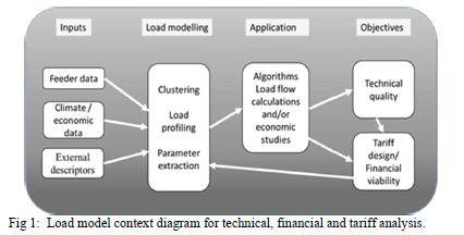
The process of developing the load models begins with preparing the inputs for defining and extracting the parameters. Clustering algorithms are applied based on the extracted parameter to classify loads and allocate representative profiles to the different classes. The load models can then be used as inputs to various application algorithms to achieve the technical, financial and tariff objectives as depicted in Fig 1.

A. Data Selection and pre-processing

The first step in developing the load models is to select and process the measurement data.

1) The data selection

The selection of data includes filtering to ensure that there are no personalized information or errors. The data contained variables such as economic class, Standard Industrial Classification (SIC), and location, which were retained as these were expected to be relevant.

2) Data sampling

A customer's measurements, based on 30 minutes intervals, contains a minimum of 17520 data points. To process customer data for all customers in the databases of large distribution companies such as Eskom and the South African municipalities would be computationally expensive. Stratified sampling, a class of probability sampling methods, was used to reduce the data processing burden. Stratified random sampling is preferred because it can be generalised, the data variability can be explained, and there is no unexplained bias in the samples [43]. Data is divided into sub-groups (strata) sharing common characteristics and each stratum representing different sections of the target population is sampled separately [43], [44].

A summarised procedure for applying stratified sampling is as follows:

• Filter data for MV feeders only (6.6kV or 11kV to 33kV)

• Select the stratum (activity class e.g. agriculture, industrial, etc)

• For each stratum

- Calculate the total power consumption as the sum of all loads within the stratum (Activity class)

- Calculate the proportion of each member (SIC) of the stratum

- Multiply this proportion with the required sample size

• Go to the next stratum

• Indicate how many samples per SIC.

After drawing the sample, the data were normalized.

3) Normalization:

The interest is in extracting the shape parameters of the load profiles. The sample contains different types and sizes of loads. Data normalization is used to eliminate the impact of large values by normalising all values to the same scale. A commonly used normalization techniques is the min-max normalisation, see eq. (1), [47] was used. The normalised data point is (Pj) of the data Pi is

where

• (Pmin) is the minimum value of power over a defined period, and

• (Pmax) is the maximum (peak) power over the period. This normalization procedure has the advantage of providing a dataset free from the effects of outliers and missing data. The normalised data are the inputs to the clustering process.

B. Load parameters identification

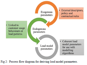
In South Africa, two seasons are pre-defined for studies and tariffing, that is, the winter (high demand) and summer (low demand) and these seasons are linked to the weather, which can be considered a parameter of external origin and hence an exogenous parameter since it cannot be controlled. The following propositions are made to differentiate between the exogenous parameters and the endogenous parameters.

Proposition 1: Exogenous parameters are parameters that are linked to weather, location, and economic parameters. These are parameters that are not derived from the same data used for load model development and are specified a-priori. These parameters include seasonality, SIC, Living Standards Measure (LSM) at an elementary level of domestic loads, and time of use periods.

Proposition 2: Endogenous parameters are parameters that are derived directly from the same data that is used for load model development.

Fig. 2 shows the process flow of deriving both the exogenous and endogenous parameters. These parameters lead to the formation of the load parameter models for the desired applications in technical, financial and tariff analysis.

 

 

Ballanti & Ochoa [45] found that the classical constant ZIP load models either underestimated or overestimated the network power losses in both winter and summer seasons and concluded that time-varying load models should be used. This finding suggests that the TOU intervals and seasonality need to be considered.

1) Exogenous parameters

Exogenous parameters may provide predefined time intervals for which parameters have to be estimated. Profiles of the different customer classes are shown in Fig. 3. These are typical profiles that form the basis of the TOU tariff structure used in Eskom.

 

 

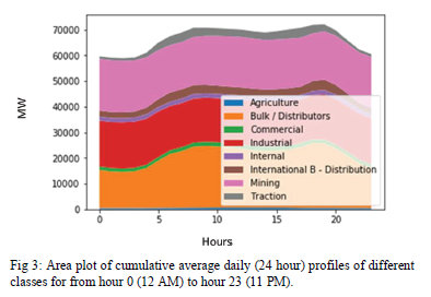
Using Fig. 3, the TOU framework is defined as follows: Peak between 7:00 and 9:00, and 18:00 to 20:00, Standard - from 9:00 to 18:00 and the remainder of hours are Off-Peak, for weekdays. For seasonality, the predefined periods for high demand season is May to July, and the remainder is low demand season. Other exogenous parameters are the Weekdays, Saturdays and Sundays. Holidays are treated as Saturdays

2) Endogenous parameters

In the literature review on LV networks, it was suggested that the active power is adequate for analysis and planning studies [13], [14]. However, this is not the case for MV network models, due to the significant presence of inductive loads. Therefore, power factor needs to be considered in MV feeder modelling [15].

The literature indicated that utilities prefer customers with high load factors, with lower energy production costs and higher system utilization, over those with low load factors. The higher load factor means indicates less variation in the load profiles. It was found that the load factors and the nighttime demand levels are the most relevant parameters to describe the customers' usage [46].

Therefore, for technical and tariff analysis, it is important to know the demand levels, time and duration of the demand for each customer. The normalized parameters derived from the above principles are expressed as:

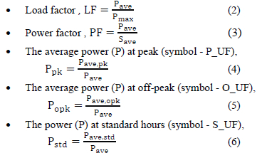
Where, P_ave: is the average half-hour active power demand in kW. P_min(P_max) is the minimum (maximum) half-hour power demand of the representative day. Pave,pk, Pave,opk, Pave.std-' are the average half-hour power demand during daily peak ,off-peak and standard periods and S_ave is the apparent power in kVA.

3) Parameter estimation using PCA method

The Principal Component Analysis (PCA) algorithm is able to reduce the vector dimensions of data while maintaining the desired variability that distinguishes the load curves [47]. Silipo [47] favoured the PCA technique, after reviewing a number of the dimension reduction techniques used in the data analytics landscape. The PCA algorithm used in this study is based on the covariance and the singular value decomposition (SVD) technique. The PCA algorithm transforms a given data set X^p into an alternative data set, Y^l, with a smaller dimension, where variables p are parameters of a dataset x^P_i £X^P. The procedure is as follows:

1) Calculate the covariance matrix

2) Determine the eigenvectors and eigenvalues

3) Rearrange the eigenvectors and eigenvalues: Sort the columns of the eigenvector matrix and the eigenvalue matrix in order of decreasing eigenvalues.

C. Classification process

Fig. 4 shows the process flow diagram followed in the classification of MV feeders. The flow diagram also depicts the modelling decisions including the selection of MV feeders or all feeders and the modelling goal. The goal could be to model typical days or the classification of feeders where there are multiple dimensions, and a decision is made to reduce them using PCA.

 

 

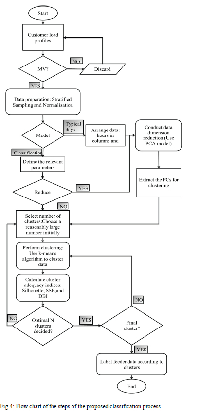
When selecting the optimal number of clusters, the initial step is to assume a large number of clusters and use the adequacy measures to aid the selection of an optimal number. There is a decision block to assess if the optimal number has already been decided and if not, the clustering process is repeated.

1) Step 1: Segmentation of load curves

In this step, the load curve is segmented based on TOU periods. The process begins by defining the load curve for a period H, as P = (P,,h = 1,..., H}. The load segment is P_T C P for τ = T. , and T corresponds to the total number of hours. Since the tariffs are modelled for typical days, H is 24.

The datasets belonging to different segments of data are identified by assigning Peak, Standard and Off-peak to the median of each of the segments. The data is separated into high demand (May to July) and low demand months (August to April).

1) Step 2: Unsupervised clustering of load data

The k-means clustering algorithm is used in grouping load profiles together using normalised parameters calculated using Eq. 1 in section II (A). The k-means framework as described in [27]-[29] and its application is summarised below:

• Assume a set of M consumers to be classified and the load of consumer m = {1,...M} is denoted as Ph^(m) and h={1 ,.. .H} denotes a time domain of the profile.

• The dataset including the load patterns is denoted as X = {x^(m),m = 1,...,M} is used to obtain a vector x.

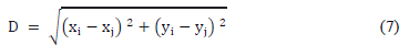
• The clustering procedure groups the M input vectors in K clusters C^(k) εX for k = {1,...,K}. The procedure uses average Euclidean distance, Eq (7):

D. Cluster Adequacy measures

Various adequacy measures can be used to determine the optimal number of clusters and assess their quality. The elbow method is popular for estimating the optimal number of clusters, but it does not always give clear results, especially when clusters are close to one another [48], so it is often used with other measures. Silhouettes scoring [49] is reported to give comparatively good performance, particularly for predicting the optimal number of clusters [50]. The Davis Bouldin index (DBI) [51] measures the internal cohesion of clusters. The silhouettes and DBI have been found to outperform other adequacy measures [48], [51]. A combination of these measures, and good visual judgement, can be effective for choosing the optimal number of clusters, with good internal cohesion and external (neighbouring cluster) isolation [52].

1) Elbow method

The Elbow method [48] plots the total of the within-cluster Sum of Square Errors SSEk as a function of the number of clusters. The elbow is a point where an increase in the number of clusters does no longer have a significant impact on the sum of square errors SSEk. The process is:

• Compute clustering algorithm (e.g., k-means clustering) for different values of k, such as for 1 to 20 clusters.

• For each k, calculate the within-cluster sum of square errors using Eq (8):

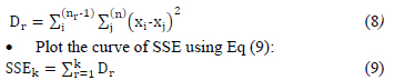
According to the number of clusters k.

• The location of a bend (elbow) in the plot is generally considered as an indicator of the appropriate number of clusters.

2) Silhouette statistic

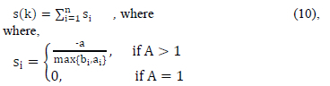
The silhouette statistic, measures how well all the objects x_i for i = 1, . n have been classified on average using Eq (10).

and (-1 < s_i< 1).

Silhouette coefficients near 1 indicate that the sample is far away from the neighbouring clusters. A coefficient of 0 indicates that the sample is on or very close to the decision boundary between two neighbouring clusters and the negative values indicate that those samples might have been assigned to the wrong cluster. To construct the silhouettes, the interest is only on the partition obtained (by the application of some clustering technique) and the collection of all proximities between objects.

3) Davis Bouldin index

The DBI is used to evaluate clusters based on internal cohesion. The measure does not depend on either the number of clusters analyzed or the method of the partitioning of the data and can be used to guide a cluster seeking algorithm [49]. To determine the DBI the distance measure should be determined. The similarity measure is calculated using Eq (11) as:

where M_ij is the distance between vectors chosen as parameters of clusters i and j, and S_i and S_j are the dispersions of clusters i and j.

The DBI measure of interest is the average from Eq (12):

A lower measure R_i is desirable as it indicates the compactness of the clusters.

E. Determining the representative profiles

A simple approach to determining the representative profiles is to allocate the average of the profiles in each cluster. Alternatively, the centroid of the cluster is used as a class representative profile. The average profile is:

where h={1,.H} is the time domain. The derivation of the clusters is illustrated in the next section.

 

III. STUDY RESULTS

A pilot study was conducted using the actual measurement data from the Eskom MV90 system and a national sample was created. The sample comprises 783 000 represented customers after applying stratified sampling and grouping customers per account from over 4 million records. These records cover about 160 SIC sectors across the country. Table 1 shows the number of samples per customer class or sector. The Eskom MV feeder measurements data strata were defined according to category variables. In each customer class, several SICs further distinguish and categorize customers. A sampling technique, which ensured all members of the stratum had the same probability of being drawn, was used to draw samples.

 

 

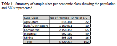
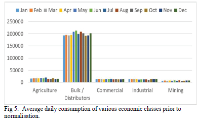
Fig. 5 shows the power consumption, in kWh, supplied (kWh_EXP) for MV feeders categorized according to economic class. The large difference between average consumptions for different classes in the database may affect the classification models. The bulk/distributor feeders dominate all others in terms of the power demand, potentially distorting the results. Since the interest is on the shape parameters of the load profiles, the domination of one customer over the others may be eliminated by normalizing the data.

 

 

A. Normalisation:

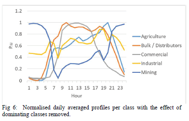
The results of normalization was achieved using Eq.(1). A selection of the normalised profiles for the different classes are shown in Fig. 6 below. All classes can be compared and analyzed from the same scale when using the normalised dataset. The profiles are normalized to values between 0 and 1.

 

 

B. Typical day load model

The objective of a typical day load model is to classify similar load profiles and associate them with the days of the week that they represent, so that the whole year can be modelled with a few typical day profiles. The common typical day models used by utilities are premised on each day of the week being distinguished by the activities that take place. The use of a clustering algorithm provides a less subjective and more scientific approach to classifying days and provide typical day profiles that share common parameter.

1) Parameters for typical days

In a typical day model, the interested is in twenty-four-hour profiles that differentiate the days, and not on specific parameters within the profiles. Therefore, each of the hours may be assumed as a parameter, and this results in 24 parameters. To represent these parameters in a scatter plot and project them in a 3-dimensional space, the PCA algorithm discussed in section II (B) was used. Three PCs achieved a representation of an average of 75% for a 24-hour profile. In Western Cape, the first three PCs account for 92% which is the highest of all provinces and in Mpumalanga three PCs account for only 60% variability.

2) Classification of weekdays

The clustering algorithm uses the PC in multiple iterations to determine the optimal number of clusters required to classify the load profiles. Following the process, in Section II and Fig 4 above the first iteration assumed a fairly large number of clusters, and in this case, the initial number of clusters was set to 20 and was reduced after assessing the results of each iteration. The elbow diagram, the silhouettes scores and the results suggested that a maximum of 3 clusters would be optimal.

3) Clustering results and validation

Fig. 7 shows the silhouettes score graph and the scatter plot of the parameters after the final iteration of clustering. The scatter plot is projected on a 3D graph. The intention of the plot is to show the results of 3 clusters in both the silhouettes and the scatter plots. The different clusters are represented by the colours.

 

 

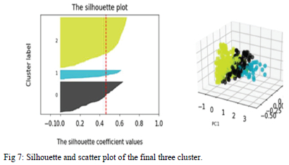
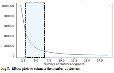
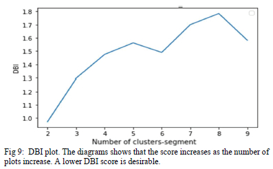
The silhouette plot shows that the clusters are clearly separate from each other without overlap since all the scores are positive. However, when there were 4 or more clusters cluster 0 had negative scores, indicating the overlap with other clusters. Fig. 8 and Fig. 9 depict the elbow and DBI plots. The elbow diagram indicated that the least square error is obtained with 3 or more clusters while the DBI suggests that lower numbers of clusters are preferred for cohesion. The shaded area is the saturation area and it is where the optimal number of clusters lie. The compromise choice is to use 3 clusters.

 

 

 

 

4) Analysis of typical day load modelling results

Table 2 shows the results from allocating the days of the week to clusters for both the winter and summer seasons as represented by the letters w and s respectively. In the weekdays' column, day, 1 is Monday. The percentages in the cluster columns 0, 1, 2 are the allocation proportions of the day-of-week profiles. in each of the clusters.

 

 

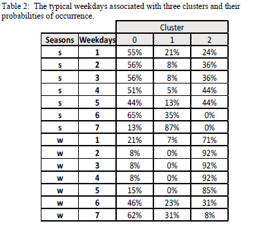
The results from table 2 show different load profiles for various typical days and that there is a seasonal impact. This means that instead of using 365 hourly profiles, two profiles can be used for summer and two profiles can be used for winter as follows: cluster 0 can be used to represent weekdays, cluster 0 or 2 may be used for Saturday and Sundays could be modelled using cluster 1 in summer. For winter season, weekdays can be represented by cluster 2 profile, and Saturday and Sunday can be represented by cluster 0. The higher percentage associated with cluster 0 means that the day can be represented using the cluster 0 profile. Similarly, with other weekdays.

The typical day clusters presented in Fig. 10 indicate that the winter weekdays can be represented by cluster 2 load profile and cluster 0 profile will be suitable to represent the weekends. The plot also shows that clusters 1 and 2 in summer are almost equivalent with minor differences only. The cluster representative load profiles were determined using Eq (13).

 

 

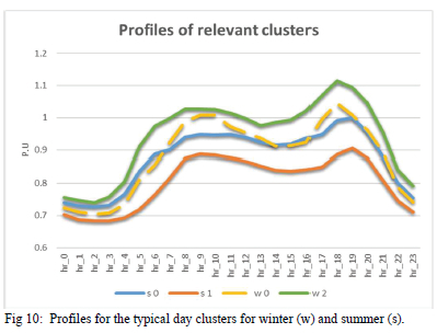
However, the results suggest that Sundays can be associated with cluster 1 and all other days can be represented by cluster 0. The results suggest that the loads in the databased can generally be represented using 4 load profiles as indicated in Fig 10. The winter weekdays can be represented using to clusters 0 and 2 while clusters 0 and 1 may be used for summer weekdays. The cluster zero for winter is represented by a yellow dash line and the blue line is for summer

C. Customer classification load model

The load model for classifying customers also follows the process as described by the flow diagram in Fig 4 above.

1) Parameter estimation

The values of the parameters were calculated using equations (2) to (6).

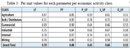
For example, in Table 3, the agricultural loads can be interpreted as having a load factor of 67%, an average power factor (PF) of 0.85 and normalised peak (P_UF), standard (S_UF) and off-peak (O_UF) parameters of 0.59, 0.61 and 0.51 respectively. The process steps stated in II (C) were followed to determine the clusters.

 

 

The problem of solving multi-dimensional vectors arises because there are 5 parameters to project and use in the clustering algorithm. To use k-means clustering, the dimensions are reduced using PCA method. In this case, the reduction is from five parameters to 2 principal components (PCs). The PCs used accounted for 88.5% the variability of the load profiles.

D. Cluster validation

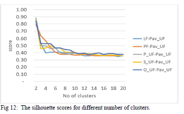
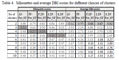
Cluster validity evaluation tools used to define the number of clusters and validating the results are Silhouettes, DBI and the elbow methods. Assuming a silhouette score threshold of 0.5, the number of clusters based on parameters LF requires three clusters, according to PF and P_UF there should be four, and using S_UF and O_UF, there should be five clusters. The elbow point analysis suggests a saturation area, determined visually, as being between 3 and 7 clusters, illustrated in Fig 11. The silhouette scores illustrated in Fig. 12 and Table 4 suggest three to five clusters are preferred. The average DBI scores in Table 4 point towards only two clusters, with scores peaking between four and seven clusters

 

 

 

 

E. Classification results

The statistical summaries of the results for five clusters are shown in Table 5. The smallest standard deviation is desirable as it indicates how the data points represented are closer to the mean. The results indicate that the clusters differ based on the shapes of their distributions as indicated by the kurtosis and skewness coefficients. Clusters 0,3 and 4 are flatter whereas the others are peakier as indicated by the kurtosis. Cluster 2 is skewed to the right and the rest of the cluster are skewed to the left.

 

 

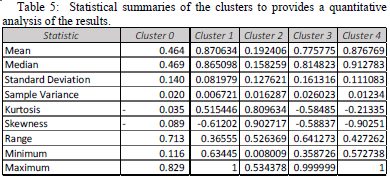
The results indicate that there are sub-classes within each economic class. The average profile of the economic class as the class representative profile may not represent adequately all customers in that class.

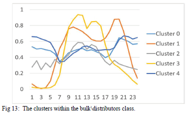
The approach for allocating Profiles were allocated to the clusters as explained in Section II (E). The bulk\distributors class with its sub-classes are shown in Fig. 13. The bulk\distributors class represents energy sold to municipalities and contains a mix of all classes including the residential class.

 

 

The average profiles of the agricultural, commercial and industrial are shown Fig. 14, Fig. 15, Fig. 16.

 

 

 

 

 

 

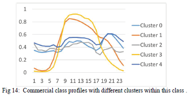
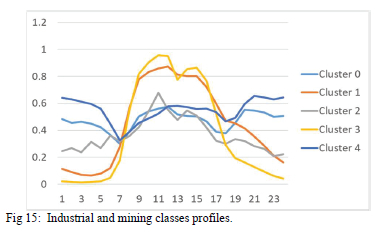
The profiles indicate that there are differences in the usage patterns of some of the customers within the same classes and that can be linked different activities and energy efficiency measures mentioned in the introduction.

In Fig 14 and Fig 15 below, clusters 1 and 3 may be linked daytime activities such as air-conditioning and the use of office equipment that begin in the morning and ends in the afternoons.

The other profiles may be linked to the malls and shopping complexes, which tend to have mild activities during daytime and peak in the evening as lighting is increased and occupancy of the hotel rooms increase

In Fig 15 most of the operations take place throughout the day with dips that could indicate a change in shifts

 

IV. Validating the results

The cluster validity tools used to define the number of clusters, such as the silhouettes, DBI and the elbow methods, were used to determine the number of clusters. The model would be valid if the identified parameter models can be implemented in practice to separate customer based on their load profiles into different clusters and ensuring that there is coherence in the parameter of the customer profiles within the same cluster.

The model validation can be achieved by evaluating the performance of the clusters using statistical tools and comparing the load profiles from the different classes. Regression analysis and analysis of variance (ANOVA) were conducted to determine the validity of each cluster. The data was then arranged per customer class with each parameter being the independent variable, and the average consumption of the customer is assumed to be the dependent variable.

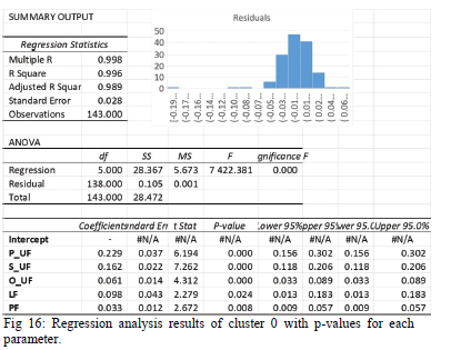
The results of the regression analysis are presented in Fig 16. As indicated by the adjusted R-square, which is close to one, the results show that the class is well explained by the parameters. Using the widely used p-value threshold of 0.005, the variables whose p-values are greater than the threshold cluster 0 are parameters LF and PF. The bar plot on the top right of Fig 16 shows that the residuals were concentrated around 0.007 and 0.011, which are sufficiently small to indicate the acceptable performance of the model. The results for all the clusters were evaluated similarly.

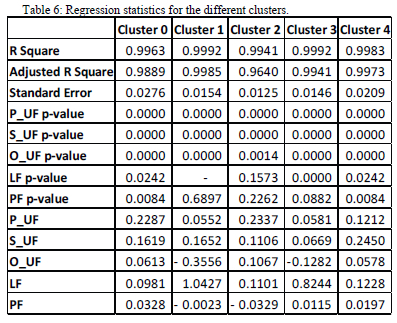
Table 6 shows the results for all 5 clusters and the summary of the regression results. The table summarises the regression results of the different parameters as well as their significance (as indicated by the R-square and p-values) in the models of each of the clusters. There is a significantly stronger relationship between the parameters and the average demand of each cluster as indicated by the smaller p-values. This indicates that these clusters are valid based on the data used.

 

 

V. Conclusions

A pilot study of customer clustering using a sample from Eskom's MV customers database shows that a set of coherent load parameter models can be extracted. Unsupervised k-means clustering was not adequate for the classification of load profiles. However, classification is improved when the algorithm is supervised using exogenous (external) parameters Analysis of the economic classes suggest that there are sub-clusters within the classes derived based on economic activity.

The research indicates that one set of load models can be applied consistently to technical, financial and tariffs analysis, avoiding the discrepancies between studies based on different load models for each application.

As expected, most clusters reflect distinct time-of-day load patterns and some show effects likely to arise from the TOU tariff periods. Therefore, if the tariffs or their associated time periods change, the cluster profiles may also change.

 

REFERENCES

[1] H. Renmu, M. Jin, D.J Hill, "Composite Load Modeling via Measurement Approach". IEEE Trans. On Power Systems, vol. 21, no. 2 , pp. 663-672, May 2006.         [ Links ]

[2] B. Prusty, D. Jena, "A critical review on probabilistic load flow studies in uncertainty constrained power systems with photovoltaic generation and a new approach," Renewable and Sustainable Energy Reviews, Elsevier, vol. 69(C), pages 1286-1302, March 2017.         [ Links ]

[3] R. Granell, C. J. Axon and D. C. Wallom, "Clustering disaggregated load profiles using a Dirichlet process mixture model," Energy Conversion and Management 92, pp. 507-516, March 2015.         [ Links ]

[4] M.J. Chihota and C.T Gaunt, "Transform for Probabilistic Voltage Computation on Distribution Feeders with Distributed Generation," Cape Town, June 2018.

[5] R. Herman, C.T. Gaunt, "A Practical Probabilistic Design Procedure for LV Residential Distribution Systems", IEEE Trans. Power Delivery, vol 23, pp. 2247-2254, April 2008.         [ Links ]

[6] E. C. Bobric, G. Cartina, G Grigoras., "Clustering Techniques in Load Profile Analysis for Distribution Stations.", Advances in Electrical and Computer Engineering vol 9 no. 1, pp. 63-66, Feb 2009.         [ Links ]

[7] C.T. Gaunt, R. Herman, H. Kadada,"Design Parameters For LV Feeders to meet Regulatory Limits of Voltage Magnitude",International Conference on Electricity Distribution (CIRED), Frankfurt, Feb 2011.

[8] D. I. H. Sun, S. Abe, R. R. Shoultz, M. S. Chen, P. Eichenberger and D. Farris, "Calculation of Energy Losses in a Distribution System", IEEE Trans. Power Syst, vol. PAS-99, pp. 1347-1356, June 1980.         [ Links ]

[9] G. Kourtis, I. Hadjipaschalis and A. Poullikkas, "An overview Of Load Demand and Price Forecasting Methodologies", International Journal of Energy and Environment, vol. 2, no. 1, pp. 123-150, Jan 2011.         [ Links ]

[10] D. Singh, R. K. Misra and D. Singh, "Effect of Load Models in Distributed Generation Planning", IEEE Trans. Power Syst., vol. 22, no. 4, pp. 22042212, Oct 2007.         [ Links ]

[11] J. H. Zhao, Z. Y. Dong, Z. Xu and K. P. Wong, "A Statistical Approach for Interval Forecasting of the Electricity Price," in IEEE Trans on Power Systems, vol. 23, no. 2, pp. 267-276, April 2008.         [ Links ]

[12] M. Soni, "Quantitative Assessment of Geographical Based Load Forecast Technique at Eskom Distribution: Forecast Error and Impact on Infrastructure Execution", 8^th South African regional conference, Cigre, 2017.

[13] C. Eid, E. Koliou, M. Valles, J. Reneses, R. Hakvoort, "Time-Based Pricing and Electricity Demand Response: Existing Barriers and Next Steps.", Utilities Policy. 2016 Jun 1;40:15-25,2016

[14] M.P. Ortega, J.I. Pérez-Arriaga, J.R. Abbad,J. Gonzalez, "Distribution Network Tariffs: A closed question?". Energy Policy. 1;36(5), pp 171225, May 2008.         [ Links ]

[15] M. J. Chihota and C. T. Gaunt, "A Transform For Probabilistic Voltage Computation on Distribution Feeders with Distributed Generation", 2018 Power Systems Computation Conference (PSCC), June 2018.

[16] C. T. Gaunt, R. Herman, M. Dekenah, R. L. Sellick, S. W. Heunis, "Data Collection, Load Modelling and Probabilistic Analysis For LV Domestic Electrification." International Conference on Electricity Distribution (CIRED), Nice, June 1999.

[17] I.A. Ferguson, and C.T. Gaunt, "LV Network Sizing in Electrification Projects-Replacing A Deterministic Method With a Statistical Method". In 17th international conference on electricity distribution (CIRED) (No. 68, pp. 1-6), 2003.

[18] T. Cousins, "Using Time Of Use (Tou) Tariffs in Industrial, Commercial and Residential Applications". TLC Engineering Solutions. 2009.

[19] Energy, D. G. "Impact Assessment Study on Downstream Flexibility, Price Flexibility", Demand Response and Smart Metering, (2016).

[20] A. Picciariello, J. Reneses, P. Frias, L. Söder, "Distributed Generation and Distribution Pricing : why do we need new tariff design methodologies ?", Electr Power Syst Res 119, pp. 370-376, Feb 2015.         [ Links ]

[21] M.J. Fell, D. Shipworth, G.M. Huebner, C.A. Elwell. Public Acceptability of Domestic Demand-Side Response in Great Britain: The Role of Automation and Direct Load Control. Energy Res Soc Sci, 9, pp. 72-84, Sept 2015.         [ Links ]

[22] Jacobs, Sharon B. "The Energy Prosumer." Ecology Law Quarterly, vol. 43, no. 3, pp. 519-579., 2016.         [ Links ]

[23] M. ElNozahy, M. Salama and R. Seethapathy, "Probabilistic Load Modelling approach using Clustering Algorithms," Power and Energy Society General Meeting (PES), Vancouver, June 2013.

[24] G. Chicco, R. Napoli, P. Postolache, M. Scutariu and C. Toader, "Electric Energy Customer Characterization for developing Dedicated Market Strategies", Proc. IEEE Porto PowerTech, Sept 2001.

[25] W. Yang, X. Bao and R. Yu, "Modeling Price Elasticity of Electricity Demand using AIDS," in Innovative Smart Grid Technologies Conference (ISGT), IEEE PES, Washington DC, 2014.

[26] G. Chicco, R. Napoli, P. Postolache, M. Scutariu and C. Toader, "Customer Characterization Options for Improving the Tariff Offer," IEEE Transactions On Power Systems, vol. 18, no. 1, pp. 381-387, Feb 2003.         [ Links ]

[27] I. P. Panapakidis, M. C. Alexiadis and G. K. Papagiannis, "Electricity Customer Characterization Based on Different Representative Load Curves," pp. 1-8, May 2012.

[28] J. A. Hartigan and M. A. Wong, "Algorithm AS 136 : A K-Means Clustering Algorithm," Applied Statistics 28, p. 100-108, Jan1979.         [ Links ]

[29] C. Fraley and A. E. Raftery, "How Many Clusters? Which Clustering Method? Answers Via Model-Based Cluster Analysis, Technical Report No. 329, Jan 1998.

[30] Y. Xu. "Probabilistic Estimation and Prediction of the Dynamic Response of the Demand at Bulk Supply Points". Diss. University of Manchester, 2015.         [ Links ]

[31] G. Tsekouras, P. Koulas, C. Tsirekis, E. Dialynas and N. Hatziargyriou, "A pattern recognition methodology for evaluation of load profiles and typical days of large electricity customers," Electric Power Systems Research 78, pp. 1494-1510, Sept 2008.         [ Links ]

[32] K. Yamashita. "Modelling And Aggregation of Loads in Flexible Power Networks-scope and status of the work of CIGRE WG C4. 605." IFAC Proceedings Volumes 45.21 , pp 405-410, 2012.         [ Links ]

[33] J.L Ramírez-Mendiola,, P. Grünewald, and Nick Eyre. "The Diversity of Residential Electricity Demand-A Comparative Analysis of Metered and Simulated Data" Energy andBuildings 151 121-131. Sept 2017:        [ Links ]

[34] A. Gbadamosi, "Dynamic Load Modelling in Real Time Digital Simulator.", 2017.

[35] V. Figueiredo, F. Rodrigues, Z. Vale and J. B. Gouveia, "An Electric Energy Consumer Characterization Framework Based on Data Mining Techniques," in IEEE Trans. on Power Systems, vol. 20, no. 2, pp. 596602, May 2005, doi: 10.1109/TPWRS.2005.846234.         [ Links ]

[36] S. Rani. and S Geeta.. "Recent Techniques of Clustering of Time Series Data: A Survey." International Journal of Computer Applications 52. pp 1-9, Jan 2012.         [ Links ]

[37] K. L. Lo, Z. Zakaria and M. H. Sohod, "Determination Of Consumers' Load Profiles based on Two-Stage Fuzzy C-Means", Proc. 5th WSEAS Int. Conf. Power Systems and Electromagnetic Compatibility, pp. 212217, Aug 2005.

[38] Lavin, A, and Klabjan, D. "Clustering Time-Series Energy Data From Smart Meters." Energy efficiency 8.4. pp 681-689, July 2015.         [ Links ]

[39] Fonseca, Jimeno A., Clayton Miller, and Arno Schlueter. "Unsupervised load shape clustering for urban building performance assessment." Energy Procedia 122, pp 229-234, 2017.         [ Links ]

[40] P. Ferraro, E. Crisostomi, M. Tucci & M. Raugi. "Comparison and Clustering Analysis of The Daily Electrical Load In Eight European Countries." Electric Power Systems Research, 141, 114-123, Dec 2016.         [ Links ]

[41] Sharma, Desh Deepak, and S. N. Singh. "Electrical Load Profile Analysis and Peak Load Assessment using Clustering Technique." IEEE PES General Meeting| Conference & Exposition, June 2014.

[42] Qiu, Wanrong, et al. "Clustering Approach and Characteristic Indices for Load Profiles of Customers Using Data From AMI." China International Conference on Electricity Distribution (CICED). IEEE, Aug 2016.

[43] A. Acharya, A. Prakash, P. Saxena and A. Nigam, "Sampling: Why and How of it?," Indian journal of medical specialities, vol. 4, no. 2, pp. 330333, July 2013;         [ Links ].

[44] . B. Kitchenham and S. Pfleeger, "Principles of Survey Research Part 5: Populations and Samples," Software Engineering Notes, vol. 27, no. 5, pp. 17-20, Sept 2002.         [ Links ]

[45] R.L. Thorndike,. "Who Belongs in The Family?". Psychometrika 18, 267-276 (1953). https://doi.org/10.1007/BF02289263.         [ Links ]

[46] P. Rousseeuw, "Sihouettes: A Graphical Aid to The Interpretation and Validation of Cluster Analysis.," Journal of Computational and Applied Mathematics , vol. 20, pp. 53-65, Nov 1987.         [ Links ]

[47] O. Arbelaitz, I. Gurrutxaga, J. Muguerza, J.M. Pérez and I. Perona. An Extensive Comparative Study of Cluster Validity Indices." Pattern Recognition, 46(1), pp.243-256. Jan 2013.         [ Links ]

[48] D.L. Davies and D.W. Bouldin, "A Cluster Separation Measure", IEEE Trans. on Pattern Analysis and Machine Intelligence, vol. 1, no. 2, pp. 224-227, April 1979.         [ Links ]

[49] K. Krzysztof, and P. Hurley. "Estimation of the Number of Clusters using Multiple Clustering Validity Indices." International workshop on multiple classifier systems. Springer, Berlin, Heidelberg, April 2010.

 

 

The research programme was sponsored by Eskom and the Department of Trade and Industry under the THRIP project.

 

 

Lolo Buys received Diploma in electrical engineering and a B.Tech. degree in electrical engineering from Tshwane University of Technology, a B.Sc. degree in computer science and information systems from University of South Africa, and M.Sc. degree in electrical engineering from University of Cape Town.
He is currently employed by Eskom Holding Soc. in Johannesburg, South Africa since 2008, as a Senior Pricing Advisor responsible for the Transmission cost of supply studies and tariff development, load and tariff data analysis.

 

 

C. Trevor Gaunt received the degree in electrical engineering from Natal University, the M.B.L. degree from South Africa, and the Ph.D. degree from University of Cape Town. He is currently an Emeritus Professor and a Senior Scholar with the Department of Electrical Engineering, University of Cape Town. He is also the Principal Investigator on research funded by the Open Philanthropy Project to investigate the mitigation of effects of geomagnetically induced currents that can introduce extreme distortion into power systems