ARTICLES

 

Improved Q-learning for Energy Management in a Grid-tied PV Microgrid

 

 

Erick O. Arwa^I; Komla A. Folly^II

^IStudent Member, IEEE; Department of Electrical Engineering, University of Cape Town, Rondebosch 7701, South Africa. His email addresses: arweri001@myuct.ac.za (Corresponding author)
^IISenior Member, IEEE; Department of Electrical Engineering, University of Cape Town, Rondebosch 7701, South Africa. His email addresses: komla.folly@uct.ac.za

 

 

---

ABSTRACT

This paper proposes an improved Q-learning method to obtain near-optimal schedules for grid and battery power in a grid-connected electric vehicle charging station for a 24-hour horizon. The charging station is supplied by a solar PV generator with a backup from the utility grid. The grid tariff model is dynamic in line with the smart grid paradigm. First, the mathematical formulation of the problem is developed highlighting each of the cost components considered including battery degradation cost and the real-time tariff for grid power purchase cost. The problem is then formulated as a Markov Decision Process (MDP), i.e., defining each of the parts of a reinforcement learning environment for the charging station's operation. The MDP is solved using the improved Q-learning algorithm proposed in this paper and the results are compared with the conventional Q-learning method. Specifically, the paper proposes to modify the action-space of a Q-learning algorithm so that each state has just the list of actions that meet a power balance constraint. The Q-table updates are done asynchronously, i.e., the agent does not sweep through the entire state-space in each episode. Simulation results show that the improved Q-learning algorithm returns a 14% lower global cost and achieves higher total rewards than the conventional Q-learning method. Furthermore, it is shown that the improved Q-learning method is more stable in terms of the sensitivity to the learning rate than the conventional Q-learning.

Index-Terms: Electric vehicle, energy management, microgrid, reinforcement learning, Q-Learning

---

 

 

I. INTRODUCTION

GRID-TIED renewable energy sources (RES) based electric vehicle (EV) charging stations are an example of a distributed generator behind meter systems (DGBMS). DGBMS is an electricity supply scheme where a renewable energy generator produces electrical power for on-site use [1]. This architecture is enabled by the application of smart metering systems, distributed generation technologies, bidirectional power conversion infrastructure and smart energy storage schemes that characterize the smart grid paradigm [2], [3], [4]. DGBMS are associated with several stochastic variables to be considered in each decision step when performing a day-ahead power scheduling [2]. These variables include the charging station's load profile, the RES generator's day-ahead output profile and the utility grid's tariff profile. This high level of randomness in a DGBMS setting makes energy scheduling and management a challenging task. The role of an energy management algorithm in such a setting is to perform an optimal temporal arrangement of the system's resources to achieve the system's objectives and maintain its overall health [4]. Specifically, the algorithm is designed to decide which of the system's energy resources should produce power, how much power they should produce and when in order to meet the system's load at minimum cost.

Various algorithms have been developed in the past to manage energy in DGBMS setups. Linear algorithms such as linear programming and mix-integer linear programming have been used to obtain solutions efficiently in less complicated spaces, but are limited in handling stochasticity [5], [6]. Also, global search techniques such as genetic algorithm (GA), particle swarm optimization (PSo), etc., have been used in literature for microgrid energy management [7], [8]. These methods perform better than linear optimization algorithms due to their ability to handle stochastic system variables. However, they are generally slow and are incapable of handling online dynamic operation.

Reinforcement learning is a reward-motivated solution mechanism. Due to their learning component and the ability to generalize solutions, reinforcement learning techniques are known to have the capability to deal with dynamic stochastic problems more easily than most optimization methods [9], [10].

Q-learning is one of the most popular reinforcement learning methods due to its simplicity, versatility and guarantee of convergence [2], [11]. It employs off-policy temporal (TD) difference update rule, i.e., updating an estimated value with another estimated value that is a step ahead of the current estimate. While this kind of recursion creates instabilities with deep reinforcement learning models, it imposes less taxing computational burden than on-policy methods such as Monte carlo and dynamic programming based algorithms [11], [12]. In [9], Q-learning was applied to perform the main utility grid scheduling problems such as economic dispatch, automatic generation control and unit commitment.

In grid-connected microgrid energy scheduling, Q-learning has been used to obtain optimal day-ahead battery schedules. Kuznetsova etal. [13] implemented a two-step ahead Q-learning algorithm with a deterministic exploration method to schedule energy storage in a grid-tied microgrid with a wind-powered distributed generator (DG), but with large discretization in both the battery energy and the wind power generation. A similar model is used with a 3-step ahead learning by Leo et al. [14] to schedule a BSS in a grid-tied PV/battery system, where the authors reported an improvement in the utilization of the PV and the BSS. Foruzan et al. [15] developed a multi-agent scheme to manage energy trading between customers and energy suppliers including the utility grid, diesel and wind generators. In [16], a Q-learning is used to schedule a shared battery storage system for a community supplied from a microgrid. The study in [17] investigates the application of Q-learning in managing energy cooperation between a PV power EV charging station with the utility grid. Despite their popularity in microgrid energy management, Q-learning techniques applied to DGBMS setups have issues of poor convergence and general instability due to their high sensitivity to the learning rate. Also, defining a reward function that achieves the objective of the learning algorithm is a challenging task as there is no conventional way of arriving at the best reward function for the purpose of the optimization task. In this paper, we developed an improved Q-learning method to obtain optimal schedules for grid and battery power in a grid-connected electric vehicle (EV) charging station in a 24-hour horizon discretized in steps of 1hour. The charging station is supplied by a solar PV generator with a backup from the utility grid. The grid tariff model is dynamic in line with the smart grid paradigm. First, the mathematical formulation of the problem is developed highlighting each of the cost components considered including a battery degradation cost model. The problem is then formulated as a Markov Decision Process (MDP), i.e., by defining each of the parts of a reinforcement learning environment for the charging station's operation. In the MDP development, different reward functions that can be found in the literature were considered and the behaviors of the Q-learning methods with respect to the various reward functions were investigated. The MDP is then solved using an improved Q-learning algorithm.

Specifically, this paper proposes to modify the action-space so that each state has just the list of actions that meet the power balance constraint. By properly constraining the agent's actions, it is shown in this paper that the improved Q-learning algorithm was able to return a 14% lower global cost with better use of the battery storage system than the conventional Q-learning procedure. Also, the proposed method achieves higher total rewards and displays a more stable learning behavior in terms of the sensitivity to the learning rate than the conventional Q-learning.

 

II. MATHEMATICAL FORMULATION

A. Model of the Charging Station

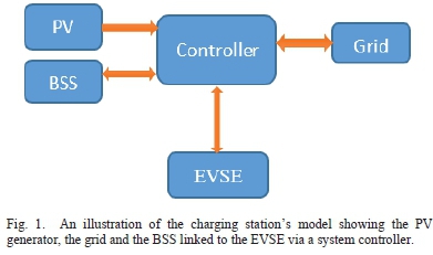
A grid-tied solar-powered EV fast CS with a battery storage system (BSS) is considered. A common DC bus is used to facilitate power-sharing among the electric vehicle supply equipment (EVSE). The DC bus is linked to the grid through an AC-DC converter and the BSS through a DC-DC converter as shown in Fig. 1. The DC bus system is preferred over the AC bus system because it requires fewer power conversion stages needed to deliver power to the electric vehicle [17]. The station supplies an electric vehicle load at the CS. It is assumed that the EV load at the CS has been forecasted and the day-ahead load profile is given.

 

 

B. Objective Function

The controller that is shown in Fig. 1 performs the scheduling of power from the various sources, namely the grid, the PV, the BSS. The station supplies an EV charging load. It is assumed that the load at the CS has been forecasted and the day-ahead load profile are known.

The purpose of this system controller is to decide, at each discrete time step, what amount of power is to be drawn from or supplied to the grid and the battery so that, in addition to the power from the PV generator, the total power is enough to supply the station's load at minimum cost. In this paper, the cost of power from the grid and the cost of battery degradation as a result of charge or discharge have been taken into consideration. The main assumptions in the development of the cost function are as follows:

1) No power is lost in the power electronic interfaces; thus, the efficiency factor for all power conversion operations is 1.

2) Both the battery charge and discharge efficiency factors are 1, thus, the two processes are lossless.

3) Power electronic conversion is instant, therefore, there is no delay between the time a power value is recommended by the system controller and the time the power is delivered to the required component.

The above assumptions are a result of practical inefficiencies of the power electronic interface. The efficiency of the power electronic interface is a function of the charging current. The study in [18] describes a practical implementation of a 75 kW EV charging equipment. The authors demonstrated that at this power level, the efficiency of the converters implemented was 99.33%. Therefore, the above assumptions do not create a significant departure from reality.

The initial battery state of charge (SoC) may be estimated using open-circuit voltage measurement. During the rest of the operational time, the SoC dynamics are described according to (1).

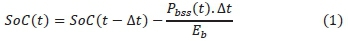
Where SoC(t), t, Δt, P_bss(t) and E_bare the instantaneous state of charge, time, size of the time discretization step, battery power and the battery energy at full charge, respectively. The state of energy (SoE) of the BSS at any time t is given by:

The instantaneous power balance equation that guarantees that the load demand is met is given by:

where P_cl(t), P_bss(t), P_g(t)>P_pv(t) are the instantaneous values of the load, the BSS power, the grid power, and the PV generator output respectively. P_bss (t) and P_g (t) are taken to be positive when injecting power to the common DC bus and negative when drawing power from the bus.

The total operational cost (C_tot) is the sum of the cost of power purchase from the grid, C_Pg (t), and battery degradation cost, Cp_hss(t) throughout the 24-hour optimization horizon, T. The objective function is, therefore, given as:

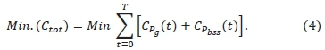
Equation (4) is subject to the constraints of power balance at the DC link given by (3), state of charge boundaries, SoC_min< SoC(t) < SoC_max, where SoC_minand SoC_maxare the upper and lower state of charge boundaries respectively; grid power limits, P_g^min< Pg(t) < P_g^max, where P_g^minand P_g^max, are minimum and maximum instantaneous grid power. The grid power limits are subject to a contract signed by the charging station owners and the grid operators.

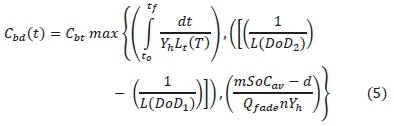
The cost of power from the grid is given by C_Pg(t) = Gt(t) Pg(t)Δt, where G_t(t) is the instantaneous grid tariff. The cost of drawing power from or storing power in the BSS is assumed to be the same and is given by C_Pbss(t) = P_bss(t)C_bd(t)Δt, where C_bd(t) is the cost of degradation of BSS per kWh given in equation (5).

To model the cost of battery degradation, the cost contributions of temperature (T), C_T, depth of discharge (DoD), C_DoDand the average SoC (SoC_av), C_SoCwere taken into account. The degradation cost is given by, C_bd(t) = max[C_T, C_DoD, C_SoC}. The equations for each contribution have been derived in [19] and [20] as shown in equation (5). In Equation (5), C_btis the battery capital cost per kWh, t₀and t_f are initial and final battery operation time for charge or discharge operations, respectively, Y_his the number of hours in a year, L(DoDj) is the cycle life of the battery at DoDj, L_t(T) is the battery life as a function of battery ambient temperature [21], Qfade is the capacity fade at battery end of life, SoC_avis the average SoC and m, n and d are curve fitting constants. The degradation equation has been derived in [19]. The max operation returns the highest value in a set of values.

 

III. MARKOV DECISION PROCESS MODEL

An MDP consists of a set of states within a predefined state space and a set of actions defined for each state and is normally used to formalize chronological decision making. For every state, there is a known stationary state transition function (or probability) that leads the agent to the next state once it takes an action in the current state [22]. Also, for every action, there is a defined reward (reinforcement) function that measures the immediate value of the action taken. The reward function holds the objective of the agent at every state [2], [17]. In this case, the reward is related to the cost minimization function of the EV charging operation.

A. State and State Space

The state, x_kof the system is the set [k, P^k_pv, G^k_t,E^k_b], where k is the time component: k = 0,1, ...,T - 1, where T is the optimization horizon, P^k_clis the EV load at the CS at time k, P^k_pvis the forecasted solar PV generation at time k, G^k_tis the forecasted grid tariff at time k, while E^k_bis the SoE of the BSS. The state space is therefore given by a union of all the individual state sets in the optimization horizon: x = ^x₀Ux₁U,...,U ^XT-1^.

B. Action and Action Space

An action represents the decision that the agent is supposed to make at any given state. Every state has a list of allowed decisions that define the action space for that state. Conventionally, battery scheduling using the Q-learning approach defines action space in two major ways.

1) The battery can be modelled to only have three possible control actions, namely, charge, discharge and idle [23], [24]. If the recommended action is a charge or a discharge operation, the battery charges or discharges at full rate, otherwise if the endorsed action is to idle, then the battery power is set to zero. This reduces the action space considerably and makes the learning process simple and efficient. However, the results returned may be sub-optimal if the choice of charging rate is not properly done. This battery model is most applicable for the backing storage (main storage) in a two-level storage system as demonstrated in the studies in [23] and [25].

2) The battery energy levels (state of energy) or state of charge may be discretized from a minimum value to a maximum value in defined steps [19]. An arbitrary choice of the initial battery energy is made, then the next values of the battery energy are selected by the learning agent at every time step. The choice of the next state of energy of the battery determines the amount of power to be supplied to or drawn from the within the time step to ensure the battery reaches the selected level.

This paper proposes an action space model that varies from state to state depending on the station's available power resources and the deficit that needs to be purchased from the grid or the excess power that is to be supplied to the grid. The objective is to improve the convergence and stability of the Q-learning algorithm. The action, in this case, is defined as the decision on what amount of power is to be drawn from or absorbed by the stationary battery and the amount of power to be imported from the grid. Consequently, the action at any time step k is defined as the set

where P^k_bssand P^k_gare the battery power and the grid power for the time step k respectively. The action space for each state is, therefore, dependent on the state variables: A_k = f(x_k). Thus, possible actions are limited by the grid power and battery energy level according to: P_g^min <P^k_g< P_g^maxas well as E_b^min<e^k_b - P^k_bssΔt < E_b^max, where P_g^minand P_g^maxare the minimum and maximum grid power respectively, and E_b^minand E_b^maxare the minimum and maximum battery energy, respectively. Therefore, to define the action space for every state, the power deficit is computed using the following equation.

If ΔP_kin Equation (7) is negative, then there is excess PV generated, thus the battery or the grid or both will have negative power to maintain the power balance at the DC link. otherwise, if ΔP_kis positive, then there is insufficient PV power, therefore, the battery or grid power will have to be positive to sustain the power equilibrium at the common DC bus.

Given the value of the power discrepancy above, the algorithm computes all possible combinations of P^k_bss and P^k_g such:

The restriction of the control action space to a set of viable solutions within the boundaries of the optimization process helps the agent to avoid exploring decisions that are not candidate solutions according to the system constraints. This reduces the problem to that of looking for optimal actions within an action space that is within the boundaries and improves the convergence and stability of the learning algorithm. The overall action space is a union of the individual state-action spaces, i.e., = A₀ U A₁ U, ... ,U A_T-1.

C. State Transition

After the learning agent takes an action, there is a need for a state transition function that takes the agent to the next state. As stated before, in an MDP with Markovian property, the next state is dependent on the current state and not the sequence of actions that led to the current state. In partially observable MDPs, the agent does not have full access to states but just observations that relay limited information of the states, and the agent's experience of these observations form the agent state [26]. The next agent state may then be derived from the experience of the next observations. In this case, the MDP is fully observable. For every state, the next state is defined by the forecasted system inputs for the next time step, the current state, and action taken in the current state. The state transition is defined as: x_k+1 = f(x_k,a_k), where x_k+1is the vector consisting of the system inputs for the next state with elements of load P_cl^k+1, solar PV generation P_pv^k+1, and the grid tariff G_t^k+1 as well as updated state of energy (SoE) of the BSS given by E^k_b⁺¹ = E^k_b ± P^k_bss Δt. The state transition is hence deterministic, i.e., the same action in the same state will always lead to the same next state. The next state x_k+1is given by (9).

D. Reward

A reward is any scalar quantity that is meant to relay the purpose of the learning algorithm to the agent. Suitable "reward engineering" is essential to link the agent's actions with the objective of the algorithm [27]. The reward is defined as r(k) = g{x_k,a_k,x_k+1).

An RL algorithm does not directly learn the cost minimization policy. The policy of cost minimization is inferred using a reward function, which the agent aims to maximize. The rewards are associated with the actions that the agent chooses in the action-space (search space). Reward engineering is, therefore, a significant part of a reinforcement learning algorithm design process.

The learning process in this study intends to minimize the cost of power purchase from the utility grid and lessen the strain on the BSS by reducing the degradation unlike the previous study in [17] where the agent was learning to both minimize cost and maximize revenue from power purchase from the grid, thus, it was rewarded for selling power to the grid. Intuitively, the agent learns to minimize cost by minimizing the power import from the grid and maximizing the self-consumption of the station's PV generated power. Therefore, rewarding the agent for selling power to the grid counteracts the agent's learning trajectory.

Since in the literature there is no agreed conventional way of designing the reward function, in this paper, we investigated various rewards functions and selected the reward function that best led to cost minimization. The reward functions investigated are as follows:

1) Exponential reward function (referred to as "inverse exponential reward") used in [17]. The function has been slightly modified to represent the objective of this study. The inverse exponential cost function is given by:

2) Negative reward function, i.e., reward expressed as negative of the cost as used in [28] and is given by.

3) Inverse reward function, i.e., reward as the inverse of the cost as used in [29] and is given by.

4) Inverse squared reward function, i.e., reward as the inverse of the square of cost. This is the first time this reward function is being used and it is given by:

It should be noted that the addition of 1 in the inverse linear and the inverse squared reward functions (12) and (13) helps to avoid division by zero in situations where the immediate cost is zero which may occur when there is no charge or discharge power scheduled and no power is drawn from or supplied to the grid. Each of the above reward functions was used to obtain an episodic cost profile to select the best reward function for the optimization problem considered in this paper. Consequently, the inverse squared reward function given by (13) was selected because it returned a lower global cost compared to all the rest as will be discussed in section V part D.

 

IV. Q-LEARNING SOLUTION FOR THE ENERGY MANAGEMENT PROBLEM

A. A Brief Introduction

The goal of any reinforcement learning algorithm is to enable an agent to learn a control policy that maximizes the total reward by iteratively interacting with the environment. Q-learning algorithm enables this learning without the need for the agent to know the environment's dynamics. This is because the update rule does not depend on the state transition probabilities like is the case with dynamic programming. The agent only needs the knowledge of the current state and the list of allowable actions in that state. Each state-action twin has a value associated with it called a Q-value. This Q-value is described using the Q-function given by (14):

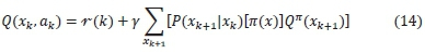
where -r(k) is the immediate reward of taking an action a_kin a current state x_k, thus, following a policy n(x) and transiting to the next state x_k+1, by a probability P. y is the discount factor that informs how much value the expected future returns have in the present. In a model-free learning algorithm, the update rule does not need the transition probability, P. Q-learning, therefore, begins by assigning an arbitrary Q-value to every state-action pair. For each episode, if the agent visits a state and takes an action, the Q-value is updated as follows:

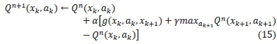
where a ε (0,1) is the learning rate which controls the extent of the modification of Q-values, Qⁿ (x_k, a_k) is the current Q-value, Qⁿ⁺¹(x_k, a_k) is the next Q-value while y ε (0,1) is the discount factor. Equation (15) means that the next Q-value of a state-action twin is substituted by the current value plus the learning rate multiplied by an error in the new estimate, i.e., the temporal difference (TD) error. The new estimate is the current reward plus the best possible Q-value in the next state. If the process is episodic and the current state is terminal, then there are no more future states in the episode, thus, the term that is multiplied by y in (15) collapses to zero during the update.

B. Conventional Q-learning Approach

In the conventional Q-learning, a Q-table is developed in as a number of states by number of possible actions matrix before learning begins and initialized by zeros (or arbitrary numbers). The action space is fixed to just one set of possible actions for all the states. The agent, thus, visits the states successively and synchronously. In each timestep, the agent visits a state and selects an action from a predefined action-space. once an action is selected in a particular state, the Q-value for the state-action pair is updated according to equation (15). For this power scheduling problem, the possible actions are the battery states of energy from the minimum value of 10kWh to a maximum value of 100kWh in steps of 10kWh. The conventional Q-learning algorithm implemented in this paper for comparison purposes is based on the studies in [9] and [11]. Its full implementation has been described in [29].

C. Proposed Improved Q-learning Approach

In this method, the Q-table is initialized as an empty hash table into which states are added as keys, with dictionaries of the allowable actions and their initial Q-values, as values. The Q-table, therefore, becomes a nested dictionary, with states indices as the main keys and an inner dictionary of possible actions as values. Each action has its Q-value initialized with zero. States are added as they occur during learning. Also, the states are not accessed sequentially as in the conventional approach. The agent does not sweep through the entire state space in each episode. Thus, the learning process occurs asynchronously. Asynchronous Q-learning enables the agent to have a delimited action space for every state. The improved Q-learning algorithm is shown in Fig. 2.

 

 

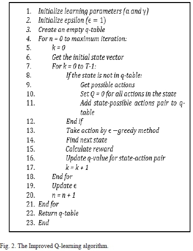
Therefore, to solve the scheduling problem using the improved Q-learning method, an empty hash table (or a dictionary data structure in Python programming) is first created. At the beginning of the learning, the algorithm reads the time and load forecast, PV generation forecast and grid tariff values for that time and returns an incomplete state vector. The initial battery energy is appended to the incomplete state vector to get a full state vector. The elements of the state vector are then joined to form a single state identity and added to the empty dictionary. If this state had not been in the table, all the possible actions associated with it are computed and all Q-values initialized with zeros. An action is chosen using the e-greedy policy and executed. The next state is then found using the state transition function. The reward is then computed using equation (13) followed by a Q-value update according to (15).

At the end of the learning process, the algorithm returns a Q-table which now contains states, possible actions and their corresponding Q-values. The process of getting the optimal action for each state using this Q-table is called policy retrieval. It is accomplished by iterating through the states in the Q-table from k = 0 to T-1. In every state, the control action that maximizes the Q-value is retrieved. Then the following states are the ones to which the selected control action leads. The states with their corresponding optimal schedules of battery power and grid power are returned.

 

V. SIMULATION RESULTS AND DISCUSSIONS

A. Input Data

To validate the developed Q-learning method, a typical solar-powered, EV fast-charging station with a maximum PV output of 70kW and a maximum demand of 80kW is considered as shown in Fig. 3 [17]. Level 3 DC fast charging analogous to an internal combustion engine vehicle filling process requires between 50kW to 100kW. Thus, the station is capable of limitedly supplying fast charging demands. The load, however, varies from time to time, with some vehicles demanding lower levels of charging rates such as level 1 (about 2kW) and level 2 (8kW to 20kW) [30].

 

 

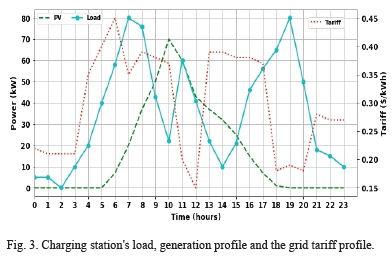
Depending on the immediate charging station's load, when the PV generation is deficient to supply the charging load, it is supplemented by the power bought from the grid and when the PV harvest is in excess, the extra energy is supplied to the utility grid. Also, as can be seen in Fig. 3, the grid tariff is dynamic. The real-time tariff profile is an effective indicator of the load demand in the grid as it rises and falls with the load demand. Therefore, the grid tariff is highest during peak load demand and lowest during off-peak hours.

The table below shows the parameters of the charging station that are input to the algorithm.

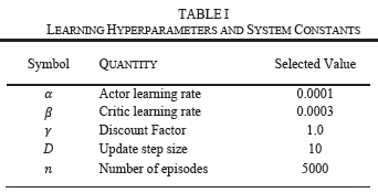
B. Learning Hyperparameters and System Constants

Table I shows both the selected learning parameters for the Q-learning algorithms and the system constants for the charging station's operation. In the e-greedy method, the greedy action is chosen by a probability, 1- ε, for εε (0,1), in any state x_k, while all other actions in the action space, A_k, are explored by a probability, ε. The exploration rate, ε, is typically initialized with a value close to 1 and as the learning proceeds, it is gradually decreased to a set minimum value, i.e., 0.1.

 

 

C. Algorithm's Learning Characteristics

Reinforcement learning algorithms are very sensitive to the learning rate (alpha). At each transition, the previous Q-value approximation is updated with the error between a new estimate and the previous guess. The value of alpha determines what percentage of this temporal difference error that is added to the previous Q-value owing to the agent's new experiences during learning. For the learning process to be stable and the convergence to be smooth, it is recommended that the value of alpha should be "sufficiently small" [9].

However, the choice of the value of the learning rate depends on the characteristics of the problem being solved such as the action space and the state space and the nature of the learning algorithm being employed. The stability of these Q-table based algorithms may be viewed from how sensitive they are to the learning rate. To test the effect of the learning rate on the Q-learning algorithms, the learning rate was increased from a 0.0001 to 0.1 in multiples of 10 while keeping all other factors such as the epsilon decay parameters and simulation variables constant.

Fig. 4 shows the learning curves for the conventional Q-learning method with different values of alpha. The horizontal axis presents the moving average rewards calculated after every 100 episodes. The graph shows that for alpha = 0.1, the average reward is oscillating, and the agent does not acquire the intended policy to maximize the total rewards. Also, some instability can be observed for alpha = 0.01, though the convergence is much smoother. Lower values of alpha, i.e., 0.001 and 0.0001 display smooth convergence with the alpha value of 0.001 converging smoothly at higher total average reward than all the rest. Thus, for this algorithm, a value of 0.001 was selected for the learning rate.

 

 

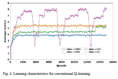
Fig. 5 shows the learning curves for the improved Q-learning algorithm for the same values of alpha as used above. An alpha value of 0.1 returned some oscillations on the average reward but the convergence was much more stable than that obtained by the conventional Q-learning. Fig. 5 reveals that the algorithm's learning curve for an alpha of 0.001 achieved the highest total rewards followed closely by an alpha of 0.0001. Therefore, for this algorithm, a value of 0.001 was selected for the learning rate as in the conventional case. Also, the curves for the various values of alpha were much closer together despite the big differences in the values of alpha. Therefore, the proposed algorithm is less sensitive to the learning rate than the conventional Q-learning method.

 

 

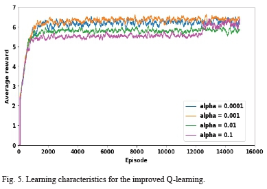
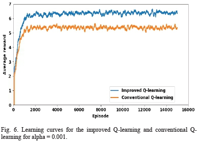
Fig. 6 shows a plot of the learning curves for both algorithms with the value of alpha set to 0.001. At this value of alpha, both algorithms converge at the highest average reward. It can be seen that the improved Q-learning method learns faster and achieves higher average episodic total rewards than the conventional Q-learning method. The proposed method converges at slightly above 6.0 while the conventional method converges at a value slightly above 5.0. This difference is as a result of the restriction imposed on the action space for each state in the proposed method. This causes it to only meet experiences that are within the power balance equation (3).

 

 

The results of this test on the effect of learning rate imply that limiting the control actions of the agent to just those that the designer knows are within the system constraints improves stability with respect to the sensitivity to the learning rate. It can be noted that the sensitivity of the algorithms to the learning rate is indicative of the confidence there is in a new Q-value estimate compared to the previous one in the TD update rule given in equation (15). If the new Q-value estimate is more likely to be inaccurate due to the unconstrained action space, that is, there is a risk of the agent veering from the objective under the current policy, or being trapped in a local optimum, then a smaller learning rate is needed to limit the extent to which the new estimates modifies the Q-values. This is what is seen with the conventional Q-learning algorithm. However, if the action space is designed to include only those values that are within both the equality and the inequality constraints of the agent's objective, then we can have more confidence that the new estimates would be more accurate, thus, a smaller learning rate may be used.

D. Effects of Various Reward Functions

A test was done to explore the behaviour of the improved Q-learning algorithm and the conventional Q-learning method under different reward functions. A moving average episodic cost profile obtained using each of the four reward functions in section III part D was plotted on the same axis for both algorithms. The moving average cost profile is a better way to compare the reward functions than the reward profile because the same objective function is used to calculate the cost in all the cases under consideration.

Fig. 7 shows the episodic cost profile for each of the reward functions for the conventional Q-learning algorithm plotted on the same axis. It can be seen that the negative reward function as given in (11) displays an unstable learning characteristic and converges at a lower average cost than all the other reward functions. This is because the Q-values were initialized by zeros while the new estimates are negative. Therefore, actions that have not been chosen always had higher Q-values than the ones that had been selected. As a result, the agent is forced to explore the search space even when the action selection algorithm (the epsilon greedy strategy) recommended exploitation. This results in unstable learning and leads to poor convergence. The other reward functions produced positive reward values, therefore, actions that have been selected had higher Q-values than those that had not been chosen. As a result, the algorithm's learning is well guided by the exploration strategy employed.

 

 

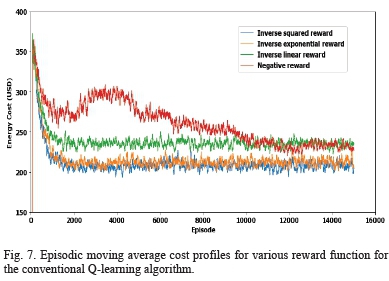
Noteworthy in Fig. 7 is the fact that the exponential reward and the inverse squared reward functions (10) and (13), respectively, converge to slightly lower global costs than the inverse linear reward function (12). This is because the inverse squared and the inverse exponential functions ensured that actions with very low costs returned very high rewards thus making the probability of them being selected much higher and effectively reducing the probability of selecting the higher cost actions. Therefore, the low-cost actions dominated the high cost actions in later episodes when more exploitation than exploration was done by the agent according to the study in [27]. The results on the global cost show that the inverse squared function produced a slightly lower reward than all the functions tested in this study. Therefore, it was selected.

Fig. 8 shows a comparative plot of the episodic cost profile for the reward functions under the improved Q-learning algorithm. It was also established that the proposed Q-learning algorithm's response to the various reward functions displayed almost a similar pattern to those exhibited by the conventional Q-learning algorithm.

 

 

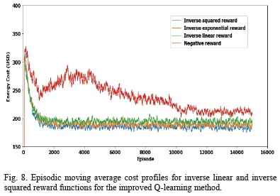
However, the difference in the global cost convergence between the inverse linear and the inverse squared function was found to be reduced while the global cost convergence difference between the negative reward and the inverse linear reward function increased. This is also attributed to the restriction of the action space in every state in the improved Q-learning method which is not the case with the conventional Q-learning algorithm.

E. Cost Convergence Results and analysis

Fig. 9 and Fig. 10 show the episodic cost profile for the conventional Q-learning and the improved Q-learning algorithms correspondingly, for 15000 learning episodes. The moving average values are calculated after every 100 episodes. It can be seen in both figures that the raw and average costs for both algorithms start at high values in earlier episodes between 0 and 2000 and decrease to lower optimized values in the later episodes beyond 2000. This is because, in both algorithms, the initial exploration rate has been set to 1.0, i.e., all the possible actions have an equal probability of being selected, thus the learning agent begins by exploring the action space because each action's probability of being selected is 1.0.

 

 

 

 

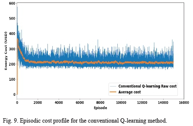
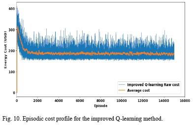
As the learning proceeds and the value of epsilon is reduced, the actions that give higher rewards, and consequently, return lower costs in each time step are selected with higher probability. With the time-step action selection getting more inclined to the optimal actions, episodic global cost converges to the optimal value according to the temporal difference control theory. Both algorithms are shown to converge at their optimal values of the global cost.

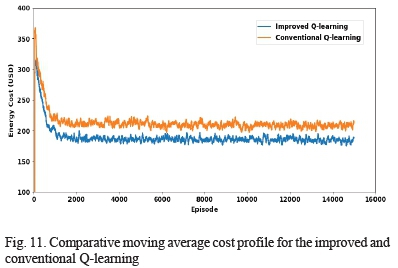
Fig. 11 shows the comparative plot of the moving average episodic cost profiles for the two algorithms during the learning phase. As can be seen in the figure, the proposed method starts at a lower initial average cost of about $320 and finishes at a value of between $200 and $150 compared to the conventional Q-learning that starts from a higher value of just above $350 and finishes at a value between $250 and $200. This is because the proposed method has its action space constrained to just the set of values of grid power and battery power that meets the load demand according to the power balance equation. Therefore, the power balance constraint, given in equation (3), is imposed before the actions are taken. As a result, its learning is constrained, thus preventing it from losing track. That is unlike the conventional Q-learning approach that uses the battery scheduling method in which the power balance is imposed only after the agent takes the action. This leads to the collection of bad experiences that causes it to lose track.

 

 

F. Optimized Power Schedule for the Improved Q-learning Algorithm

At the end of the learning period, the optimal power schedule was retrieved from the Q-table using a greedy policy. The greedy policy returns the action with the highest Q-value in every state throughout the optimization horizon. In this subsection, the power schedule derived from the optimal episode obtained from the proposed method is discussed. The cost minimization actions recommended by the improved Q-learning algorithm at various times within the episode are identified and explained. Of interest in this section is the battery utilization exhibited by both algorithms that resulted in marked differences in the battery degradation cost and the returned global cost between the proposed algorithm and the conventional Q-learning method.

In understanding the schedule, the signs of the scheduled power values of the battery and the grid should be taken into consideration. Any scheduled power is always positive when supplying the load through the common bus and negative when drawn from the bus. A negative battery power, therefore, represents a charge command while a positive battery power means a discharge command. Therefore, the algorithm ensures that a charge and a discharge operation cannot occur at the same time without the need for a secondary controller to enforce that constraint. Similarly, a negative grid power denotes a power supply to the grid whereas a positive grid power means a power purchase from the grid. Also, the battery energy transitions are occasioned by power schedule actions, thus the effect of a battery charge or discharge command in a time step is observed in the next time step.

To minimize the cost of supplying the charging station's load, the algorithm is designed to use the following strategies.

1) The algorithm maximizes the self-consumption of the PV generated power.

2) The algorithm utilizes less grid power when the tariff is high and more of it when the tariff is low.

3) The algorithm performs short charge/discharge cycles to lower the battery degradation cost.

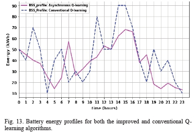
As shown in Table II, the two algorithms returned almost the same overall cost of power purchase from the grid, except for a small difference of $3. Therefore, the main difference is observed in the battery utilization, that is, the magnitude of the charge/discharge rates.

 

 

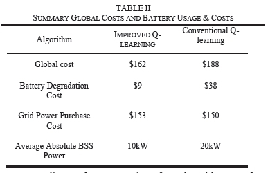
Fig. 12 shows the power schedule for both the battery and the utility grid plotted alongside the input PV, grid tariff and the charging station's load profiles. The battery energy values have been divided by the time-step constant to get kW values.

 

 

The first strategy is implemented by charging the battery when the solar PV generation is high and using the stored energy when there is low PV and the grid tariff is high. The battery and grid power are positive when supplying power to meet the charging station's load and negative when absorbing power from the station's common DC bus. It can be seen in Fig. 12 that the general trend shows a discharge from the 0 to 5^th hour (i.e, the pink curve labeled "BSS"). From the 5^th to the 7^th hour, the battery charges as PV generation rises. However, a discharge occurs from the 7^th to the 8^th hour to supply the load that peaks at around this time. From the 8^th to the 15^th hour, the battery continues to charge due to high PV generation, except for a small instability at the 12^th hour, which is expected due to the stochasticity in the environment causing some suboptimal decisions to be made by the agent. From the 15^th to the 20^th hour, the battery shows a discharge trend due to the drop in PV power and an increasing load to be supplied. Again, there is a suboptimal decision to charge at the 17^th hour.

The second strategy is executed by scheduling high grid power intake when the tariff is low and reducing the purchase of grid power when the grid tariff is high. Also, cost savings are done by generally minimizing grid power intake since the grid power cost is mostly higher than the cost of battery degradation for small power values. This, however, depends on the existing load to be supplied and the availability of PV power and the energy level in the battery. In Fig. 12, it can be seen that there is a high grid power intake between the 5^th and the 7^th hour despite the high grid tariff because, at this time, the battery energy is almost completely drained, there is low PV generation, thus the need to use the grid to supply the rising load (i.e, the black curve labeled "grid"). The grid power intake is generally low between the 9^th and the 16^th hour, even going to negative at the 10^th hour when the grid absorbs power, due to high PV generation. At the 10^th and 12^th to 15^th hour, the station supplies power back to the grid due to excess PV generation. However, power is not supplied to the grid in the 11^th hour but is drawn from it due to low tariff, which implies that the utility grid has excess generation in relation to its load.

The third strategy is implemented by limiting the size of the charge/discharge steps. Although it is expected to be more cost effecting to use all the excess PV to charge the battery, the inclusion of battery degradation cost limits the charging rate. It is therefore costly to recommend high charge or discharge schedules since the cost of degradation due to depth of discharge grows exponentially with an increase in the magnitude of charge/discharge steps [24]. Therefore, the algorithm generally recommends shorter charge and discharge cycles to protect the battery. It is in this regard that the two algorithms differ in their global costs.

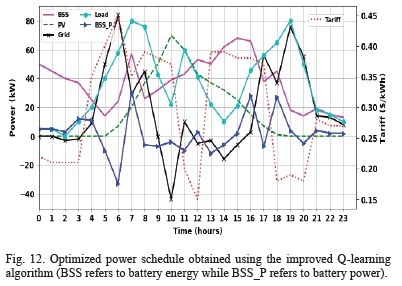
To investigate the difference in the battery charge/discharge cycles for the improved and the conventional Q-learning methods, a plot of the battery energy profiles for both algorithms was included.

Fig. 13 shows the battery energy profiles for the 24 hours of operation for the two algorithms.

 

 

It can be seen that the improved Q-learning algorithm recommends shorter charge/discharge rates than the conventional Q-learning method. The absolute battery power recommended by the algorithm at any time is calculated by getting the difference between the next battery energy level and the current value. some of the marked large battery power schedules recommended by the conventional Q-learning algorithm can be seen at the 3^rd, 10^th and 13^th hours when the recommended absolute battery power values were 40kW (i.e., a battery discharge operation from 50kWh to 10kWh), 50kW (i.e., a battery charge operation from 30kWh to 80kWh) and 40kW (i.e., a battery charge operation from 50kWh to 90kWh) respectively. The maximum absolute battery power recommended by the proposed algorithm is about 30kW (i.e., a battery charge operation from 25kWh to 55kWh) which occurs at the 6^th hour.

Furthermore, if the absolute power values recommended by the two algorithms throughout the 24-hour horizon were averaged, the average absolute power recommended by the improved Q-learning algorithm was found to be 10kW while that of the conventional Q-learning method was found to be 20kW as shown in Table II. The battery degradation cost increases significantly with the increase in the absolute power recommended by the algorithms. Consequently, the battery degradation cost for the proposed method is more than 4 times lower than that of the conventional method as shown in Table II.

When the policy was retrieved, the optimal episode for the improved Q-learning method returned about 14% lower global cost than the conventional Q-learning method as shown in Table II. This major difference is attributable to the higher cost of battery degradation resulting from the episode obtained using the conventional method than in the proposed method. There is higher degradation with the conventional method because the algorithm recommends much longer charge and discharge cycles than the proposed method.

 

VI. CONCLUSION

An improved Q-learning algorithm using an asynchronous update technique for energy management in a grid-connected solar-powered EV charging station with a battery energy storage system has been presented. In the Markov Decision Process model, the study has proposed the expression of the reward as the square of the reciprocal of the cost plus a constant. This reward function produced a slightly lower global cost than other reward functions in the literature. Also, the learning characteristics of the proposed method and the conventional Q-learning method under different values of the learning rate have been investigated. simulation results show that the improved Q-learning algorithm learns faster, is less sensitive to different values of learning rate and displays a more stable learning characteristic than the conventional Q-learning algorithm. Furthermore, analysis of the battery usage established that the restriction of the improved Q-learning algorithm's action space to the set of actions that meet the power equilibrium condition at the common bus leads to better usage of the battery energy storage and is responsible for the improvement of its stability in the learning process as compared to the conventional Q-learning. Moreover, the improved Q-learning algorithm returned 14% lower global cost than the conventional Q-learning technique.

Future studies on this problem should consider the application of deep reinforcement learning in dynamic energy scheduling to harness the full potential of reinforcement learning techniques that may not be achieved using static optimization methods such as Q-table-based reinforcement learning techniques.

 

NOMENCLATURE

Abbreviations

BSS Battery storage system

CS Charging station

DG Distributed generator

DGBMS Distributed generator behind the meter system

EV Electric vehicle

EVSE Electric vehicle supply equipment

GA Genetic algorithm

MDP Markov Decision Process

PSO Particle swarm optimization

PV Photovoltaic

RES Renewable energy source

TD Temporal difference Notations

a Action

C_bdBattery degradation cost

C_btBattery capital cost

C_DoDDegradation cost due to depth of discharge

Cp_hssBattery power cost

C_PgGrid power cost

C_TCost of degradation due to temperature

DoD Depth of discharge

E_bBattery energy capacity

G_tGrid tariff

j Depth of discharge index

k Timestep/state index

L_t (T) Battery lifetime as a function of ambient temperature

L(DoD) Battery lifetime as a function of depth of discharge

n Iteration index

P Probability

Pcl Load at the charging station

Pg Grid power

Ppv PV power

Pbss Battery charge/discharge power

Q Q-value

Qfade Battery capacity fade

Rt Battery thermal resistance

SoC State of charge

SoCav Average state of charge

SoE State of energy (battery energy level)

T Ambient temperature

t Time

x State

A. Action space

a Learning rate

Y Discount Factor

r Reward

n Policy

X State space

 

REFERENCES

[1] M. O. Badaway, "Grid Tied PV/Battery System Architecture and Power Management For Fast EV Charging," Ph.D Thesis, Department of Electrical Engineering, The University of Akron, 2016.         [ Links ]

[2] A. O. Erick and K. A. Folly, "Reinforcement Learning Approaches to Power Management in Grid-tied Microgrids : A Review," in Clemson University Power Systems Conference, 2020, pp. 1-6.

[3] X. Zhaoxia, S. Xudong, Z. Xian, and Y. Qingxin, "Control of DC Microgrid for Electrical Vehicles(EV s) Wireless Charging," in 2018 China International Conference on Electricity Distribution, 2019, pp. 2082-2087.

[4] D. E. Olivares, A. Mehrizi-Sani, A. H. Etemadi, C. A. Cañizares, R. Iravani, M. Kazerani, A. H. Hajimiragha, O. Gomis-Bellmunt, M. Saeedifard, R. Palma-Behnke, G. A. Jiménez-Estévez, and N. D. Hatziargyriou, "Trends in microgrid control," IEEE Trans. Smart Grid, vol. 5, no. 4, pp. 1905-1919, 2014.         [ Links ]

[5] N. A. Luu and Q. T. Tran, "Optimal energy management for grid connected microgrid by using dynamic programming method," IEEE Power Energy Soc. Gen. Meet., vol. 2015-Septe, no. 1, pp. 1-5, 2015.         [ Links ]

[6] D. Zhang, "Optimal Design and Planning of Energy Microgrids." Ph.D Thesis, Department of Chemical Engineering, University College London, 2013.         [ Links ]

[7] M. Hijjo, F. Felgner, and G. Frey, "PV-Battery-Diesel microgrid layout design based on stochastic optimization," in 2017 6th International Conference on Clean Electrical Power: Renewable Energy Resources Impact, ICCEP 2017, 2017, pp. 30-35.

[8] A. T. Eseye, J. Zhang, D. Zheng, and D. Wei, "Optimal energy management strategy for an isolated industrial microgrid using a modified particle swarm optimization," 2016 IEEE Int. Conf. Power Renew. Energy, ICPRE 2016, pp. 494-198, 2017.

[9] E. A. Jasmin, "Reinforcement Learning Approaches to Power System Scheduling." Ph.D Thesis, School of Engineering, Cochin university of Technology, 2008.         [ Links ]

[10] J. Wang, K. Zeb, T. Dhruva, S. Hubert, L. Joel, M. Remi, C. Blundell, K. Dharshan, B. Matt, "Learning to reinforcement learn," DeepMind, London, UK. pp. 1-17, 2016.

[11] C. J. C. H. Watkins, "Learning from Delayed Rewards," Ph.D Thesis, Department of Computer Science, University of Cambridge, 1989.         [ Links ]

[12] R. S. Sutton and A. G. Barto, Reinforcement Learning: An Introduction, 2nd ed. The MIT Press, 2018.

[13] E. Kuznetsova, Y. F. Li, C. Ruiz, E. Zio, G. Ault, and K. Bell, "Reinforcement learning for microgrid energy management," Energy, vol. 59, pp. 133-146, 2013.         [ Links ]

[14] R. Leo, R. S. Milton, and S. Sibi, "Reinforcement learning for optimal energy management of a solar microgrid," in 2014 IEEE Global Humanitarian Technology Conference - South Asia Satellite, GHTC-SAS 2014, 2014, pp. 183-188.

[15] E. Foruzan, L. K. Soh, and S. Asgarpoor, "Reinforcement Learning Approach for optimal Distributed Energy Management in a Microgrid," IEEE Trans. Power Syst., vol. 33, no. 5, pp. 5749-5758, 2018.         [ Links ]

[16] V. H. Bui, A. Hussain, and H. M. Kim, "Q-learning-based operation strategy for community battery energy storage system (CBESS) in microgrid system," Energies, vol. 12, no. 9, 2019.         [ Links ]

[17] A. O. Erick and K. A. Folly, "Energy Trading in Grid-connected PV-Battery Electric Vehicle Charging Station," in 2020 International SAUPEC/RobMech/PRASA Conference, Cape Town, South Africa, 2020, pp. 1-6.

[18] M. Badawy, N. Arafat, S. Anwar, A. Ahmed, Y. Sozer, and P. Yi, "Design and Implementation of a 75kW Mobile Charging System for Electric Vehicles," IEEE Trans. Ind. Appl., vol. 52, no. 1, pp. 369-377, 2016.         [ Links ]

[19] M. O. Badawy and Y. Sozer, "Power Flow Management of a Grid Tied PV-Battery System for Electric Vehicles Charging," IEEE Trans. Ind. Appl., vol. 53, no. 2, pp. 1347-1357, 2017.         [ Links ]

[20] C. Zhou, K. Qian, M. Allan, and W. Zhou, "Modeling of the Cost of EV Battery Wear Due to V2G Application in Power Systems," IEEE Trans. Energy Convers., vol. 26, no. 4, pp. 1041-1050, 2011.         [ Links ]

[21] K. J. Laidler, "The development of the arrhenius equation," J. Chem. Educ., vol. 61, no. 6, pp. 494-498, 1984.         [ Links ]

[22] R. Bellman, "A Markovian Decision Process," J. Math. Mech., vol. 6, no. 5, pp. 679--684, 1957.         [ Links ]

[23] V. François-lavet, D. Taralla, E. Damien, and R. Fonteneau, "Deep Reinforcement Learning Solutions for Energy Microgrids Management," in European Workshop on Reinforcement Learning, 2016, pp. 1 -7.

[24] V.-H. Bui, A. Hussain, and H.-M. Kim, "Double Deep Q- Learning-Based Distributed operation of Battery Energy Storage System Considering Uncertainties," IEEE Trans. Smart Grid, vol. 11, no. 1, pp. 457-469, 2019.         [ Links ]

[25] V. François-Lavet, "Contributions to deep reinforcement learning and its applications in smartgrids." Ph.D Thesis, Department of Electrical Engineering and Computer Science, university of Liege, 2017.         [ Links ]

[26] Y. Wan, M. Zaheer, M. White, and R. S. Sutton, "Model-based Reinforcement Learning with Non-linear Expectation Models and Stochastic Environments," in FAIM Workshop on Prediction and Generative Modeling in Reinforcement Learning, 2018, pp. 1-5.

[27] D. Dewey, "Reinforcement Learning and the Reward Engineering Principle Rewards in an Uncertain World," in AAAI Spring Symposium Series, 2014, pp. 1-8.

[28] J. Xie, Z. Shao, Y. Li, Y. Guan, and J. Tan, "Deep Reinforcement Learning with optimized Reward Functions for Robotic Trajectory Planning," IEEE Access, vol. 7, pp. 105669-105679, 2019.         [ Links ]

[29] A. O. Erick and K. A. Folly, "Power Flow Management in Electric Vehicles Charging Station using Reinforcement Learning," in 2020 IEEE Congress on Evolutionary Computation (CEC), 2020, pp. 1 -8.

[30] M. Yilmaz and P. Krein, "Review of Charging Power Levels and Infrastructure for Plug-In Electric and Hybrid Vehicles and Commentary on Unidirectional Charging," IEEE Trans. Power Electron., vol. 28, no. 5, pp. 2151-2169, 2012.         [ Links ]

 

 

This work was based on the research supported in part by the National Research Foundation of South Africa under Grants UID 118550 and 119142.
The paper is Based on "Energy Trading in Grid-connected PV-Battery Electric Vehicle Charging Station" in the SAUPEC/RobMech/PRASA 2020 proceedings", by (Arwa O. Erick and Komla A. Folly) which was published in the Proceedings of the SAUPEC/RobMech/PRASA 2020 Conference held in Cape Town, South Africa 29 to 31 January 2020. © 2020 SAIEE

 

 

Erick O. Arwa Received his BSc. degree in Electrical and Electronic Engineering from the university of Nairobi, Nairobi, Kenya in 2016. In 2015, he interned at Powerhive East Africa Ltd as a research assistant in solar energy systems design and deployment. He is currently studying for the master's degree in Electrical Engineering at the university of Cape Town, Cape Town, South Africa under the Mandela Rhodes Foundation Scholarship. His research interests include operation and control of intelligent microgrids, machine learning and power systems optimization. Erick is a student member of IEEE.

 

 

Komla A. Folly (M'05, SM'10) received his BSc and MSc Degrees in Electrical Engineering from Tsinghua university, Beijing, China, in 1989 and 1993, respectively. He received his PhD in Electrical Engineering from Hiroshima university, Japan, in 1997. From 1997 to 2000, he worked at the Central Research Institute of Electric Power Industry (CRIEPI), Tokyo, Japan. He is currently a Professor in the Department of Electrical Engineering at the university of Cape Town, Cape Town, South Africa. In 2009, he received a Fulbright Scholarship and was Fulbright Scholar at the Missouri university of Science and Technology, Missouri, uSA. His research interests include power system stability, control and optimization, HVDC modelling, grid integration of renewable energy, application of computational intelligence to power systems, smart grid, and power system resilience. He is a member of the Institute of Electrical Engineers of Japan (IEEJ), and a senior member of both the South African Institute of Electrical Engineers (SAIEE) and the IEEE.