Convergence of the fast state estimation for power systems

 

 

Md. Ashfaqur Rahman^{I, II}; Ganesh Kumar Venayagamoorthy^{I, III}

^IReal-Time Power and Intelligent Systems Laboratory, Holcombe Department of Electrical and Computer Engineering, Clemson University, Clemson, SC 29634, United States
^IIDepartment of Electrical and Computer Engineering, North South University, Dhaka, Bangladesh Email: marahma@g.clemson.edu
^IIISchool of Engineering, University of Kwazulu-Natal, Durban 4041, South Africa Email: gvenaya@clemson.edu

 

 

---

ABSTRACT

Power system state estimation is a fundamental computational process that requires both speed and reliability. To meet the needs, some variants of the constant Jacobian methods have been used in the industry over the last several decades. The variants work very well under normal operating conditions with nominal values of the states. However, the convergence of the methods are not analysed mathematically and it may contain pitfalls. In this study, the convergence of the constant Jacobian methods are analysed and it is shown that the methods fail under high variations of the states. To increase the reliability of the processes, a multi-Jacobian method is proposed. Through simulation, a special case is shown for IEEE 68, and IEEE 118-bus systems where the Jacobian calculated with the nominal value fails, and the proposed multi-Jacobian method succeeds.

Key words: Convergence, dishonest Gauss Newton method, fast decoupled state estimator, parallel programming, weighted least squares estimator.

---

 

 

1. INTRODUCTION

Proper operation of the power system largely depends on proper monitoring. State estimation is a core part of the monitoring system. The purpose of estimation is to remove errors from an overdetermined set of measurements. It yields a noise-free consistent set of state variables that is used for contingency analysis, optimal power flow, load forecasting etc [1,2]. As a large number of applications depend on the output of the estimator, it is very important to ensure it's reliability. Due to the high accuracy, Weighted Least Squares (WLS) estimator became the universally accepted solution for state estimation [3,4]. It was originally developed by Carl Friedrich Gauss in 1795 [5] and was proposed for power systems by Fred Schweppe in 1970 [6, 7]. The most time-consuming part of the WLS estimator is the computation of the Jacobian matrix. To avoid matrix inversion, Cholesky decomposition is used and it is followed by a back substitution. Though it makes the process quite fast, it is not suitable for parallel implementation [8].

One of the major variants of the WLS estimator that is very popular in the industry is the fast decoupled (FD) estimator [9]. It takes the advantage of the constant Jacobian as well as the decoupling of the real and reactive powers [10]. Keeping the Jacobian constant is generally known as the dishonest Gauss Newton method [11]. If the Jacobian is kept constant for all the samples of measurements, it is called Very DisHonest Newton (VDHN) method [12]. The FD estimator exploits the advantages of decoupling with the advantages of VDHN.

In VDHN, the Jacobian is calculated at a nominal value [13]. The calculated Jacobian is used until there is any change in the topology. Though the method is very popular, the convergence is not analysed in the literature. It may be due to the difficult nature of the multi-state nonlinear estimators.

In this study, the nature of convergence of VDHN is analysed and it is found that the constant Jacobian calculated at the nominal values may fail under specific circumstances. It is also shown that the range of convergence can easily be extended with some simple modifications. Though extended convergence takes a longer time, it can be very useful at times. The speed and the reliability can be achieved at the same time with a multi-Jacobian solution.

The analysis of convergence is shown with a single state. The issue of constant Jacobian for multi-state estimation is shown through simulation of IEEE 68, and IEEE 118-bus test systems. A single case of failure can pose a potential threat for the power system. As the advantage of the dishonest method comes with the parallel implementation, the estimations are executed on a GPU platform [14]. The main contribution of the paper is as follows,

• The nature of convergence of the dishonest Gauss Newton method is analysed geometrically for a single state. It is shown that the constant Jacobian taken at a higher slope can increase the range of convergence significantly.

• Through simulation, it is shown that the constant Jacobian taken at the flat start can work well for normal operations on the linear range. But, it fails to converge for high diversity of the states.

• A multi-Jacobian method is proposed for secure operation. It is able to withstand disturbances in the power system.

The rest of the paper is organized as follows. The backgrounds of the concerned estimation methods, i.e. WLS, and the dishonest method, are described in Section 2. The convergence of the dishonest method for a single state is analysed in Section 3. The required time for the constant Jacobian methods for different slopes are shown and a simple multi-Jacobian estimator is proposed in Section 4. A special case of failure for the nominal Jacobian is shown in Section 5. The paper is concluded with plan for future works in Section 6.

 

2. BACKGROUND

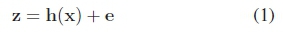
Measurements are collected from different parts of the system in the forms of power flows, power injections, voltage magnitudes, and current magnitudes [15]. The collected measurements contain errors of different levels that needs to be removed to get a clearer view of the system. Let, z denotes an m_s χ 1 measurement vector with errors. So, the relation between z, the nonlinear function of the measurements h(.), the state vector x, and the measurement error e is written as,

In power system state estimation, voltage magnitudes and angles are considered as the state variables as they form the set with minimum cardinality that can describe the whole system [3]. The angle of the reference bus is taken as the reference angle and all other bus angles are determined with respect to that. If there are N buses, the state vector x is represented as,

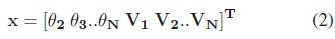
Here, θ and V, with proper subscripts, represent voltage angles and magnitudes respectively. A system with N buses will have 2N - 1 state variables. In the process of estimation, the number of measurements exceeds the number of states to form an overdetermined system [16].

The accuracy is measured by the L₂-norm of the residues that are calculated as the difference between the original measurements and the estimated measurements [17]. Minimizing the norm is the objective of the optimization problem,

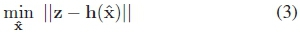
where, is the estimated state vector.

2.1 Weighted Least Squares Estimation

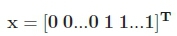
Like other nonlinear problems, WLS estimator linearises the system over a small range. Then it applies linear operations to get an updated value. The system is linearised again based on this updated value and uses the linear estimation. This process is repeated unless the estimated value converges. In this method, x is started with a close value to the solution. In the beginning, when there is no previous value, all voltage magnitudes start as 1 and all voltage angles as 0 which is known as flat start [18],

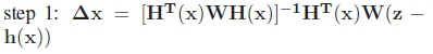
After collecting the measurements and constructing the Jacobian matrix H(x) at flat start, the following steps are repeated until the state vector converges to a solution,

•

• step 2: x = x + Δx

• step 3: update h(x) with new x

• step 4: update H(x) with new x

Here, the matrix, W denotes the relative weights of the measurements that are usually taken as the inverse of the corresponding error variances [19]. The WLS method is also known as the honest Gauss Newton method.

2.2 Dishonest Gauss Newton Method

In the dishonest Gauss Newton method, step 4 of the WLS method is not executed [11]. H is calculated for flat start at the beginning and updated after a certain period. As mentioned earlier, if H is kept constant until there is any change in the topology, the method is called very dishonest.

The constant H reduces the computation of step 1. As H remains constant, (H^TWH)^_1H^TW does not change. Therefore, a constant matrix can be multiplied with the vector z - h(x) to complete step 1. The matrix-vector multiplication is very suitable for parallel implementation on a GPU. The steps can be reorganized as,

• Before estimation: Calculate M (H^TWH)-¹H^TW for flat start

• During estimation:

  - Take previous estimation, x and new measurement set, z

  - Repeat the following steps till convergence,

    * step i: Calculate residuals, r = z - h(x)

    * step ii: Calculate Δx = Mr

    * step iii: Calculate x = x + Δx

Though the method described in [11] proposes the flat start values for calculating H before estimation, it will be shown that it is not mandatory for convergence. In fact, instead of using one Jacobian, different Jacobians can be used for handling different situations of the system such as large changes in real and reactive power flows.

 

3. CONVERGENCE ANALYSIS OF DISHONEST METHOD

Before analysing the nature of convergence of the dishonest method, it is important to illustrate the difference between the honest and the dishonest method. To make it simpler, a single variable function, y = f (x) is analysed. The applicability of this analysis on multi-variable functions will be made clear through simulations.

Let, the iterations start at x = x₀with an objective of y = yf (Fig. 1(a)). The slope at x_o is denoted with m₀. In the honest method, x₀is used with the difference between f (x₀) and yf to find the new position, x₁. For x₁, the slope is calculated as m₁and the process is repeated to find the solution.

 

 

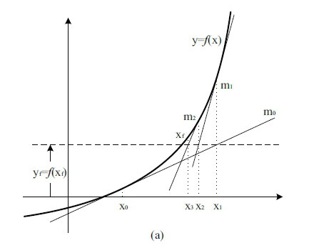
On the other hand, the dishonest method starts with a fixed slope, m. The difference is always multiplied with this constant to find the new position of x as shown in Fig. 1(b). The use of a constant slope, m does not only eliminate the calculation of m, but it also changes the division operation to multiplication (m^-1). The contribution is not significant for a single variable system, but it becomes an important improvement for multi-dimensional large-scale systems.

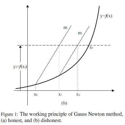
However, the dishonest method does not ensure convergence for any slope, m. The choice of m depends on the functions, the region of operations, the target values, and on the starting values. Calculating the Jacobian for the extreme target and extreme starting values can make the process slow. So, for each function, the Jacobian can be developed for a normal, and some extreme conditions. In power system state estimation, there exist a few specific types of functions between the state variables and the measurements. It is sufficient to find a suitable m for these functions. From the standard power flow equations, the major functions can be written as,

Here, the flows are measured from bus i to bus j. The measurement of current is excluded in this study. As the last two equations do not include any function, they are skipped in this analysis as well. The power injections are the combinations of power flows; so their analysis resemble that of the flows. Before jumping to the specific functions, the nature of convergence is discussed first.

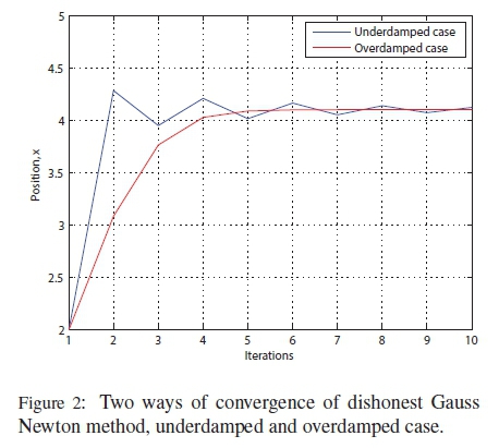
3.1 Nature of Convergence

The state can converge under two major scenarios. They are referred as the underdamped and the overdamped case. In the first case, there is an overshoot and it follows a zigzag path to reach the final value. In the overdamped case, there is no overshoot, and x changes monotonically to reach the final value as shown in Fig. 2. In some situations, a mixture of the two cases appears in the same problem.

 

 

3.2 Linear Functions

The analysis of the linear function is simple. The overdamped and the underdamped cases are shown in Fig. 3. There is no event where both cases can appear simultaneously.

 

 

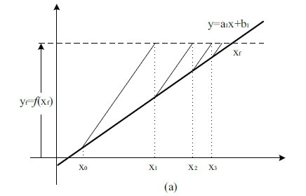
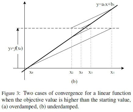
To analyse the condition for convergence, the value of m is started with the maximum. For m -> ∞, the process reduces to an incremental search method. By reducing the slope, the convergence can be made faster. It stays under overdamped case for α₁ <m< ∞, where a₁is the slope of the line. With further reduction, the process converges up to a certain limit under underdamped case. After that, it fails to converge.

Lower Limit of m: In Fig. 3(b), if the process starts with x₀to find yf = f (xf ), it changes according to the following equations,

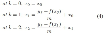
If x₂ is closer to xf than x₀, it will be able to converge. In case of xf >x₀, the condition of convergence can be written as,

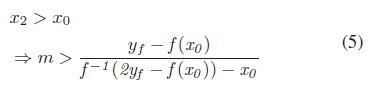
The expression of (5) is common for any system with monotonically increasing slope. For linear functions, it can be written as,

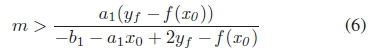
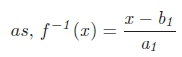
By replacing y = f (x) = a₁ x + b₁in (6), the final expression can be derived as,

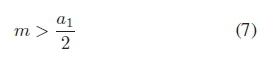
For linear functions, (7) shows that the minimum slope does not depend on the starting or the final value. It only depends on the slope of the line. If the quadratic and sinusoidal functions can be linearised over a small portion, it is also applicable for that. This is the proof why a constant Jacobian always works for a change over the linear region of the system.

However, it is noticeable that the best value for m is not the value given by (5) or (7). Using a marginal value can lead to a very large number of iterations. Those are the minimum values for which convergence can be secured. The best value for a linear function is the constant slope, i. e., m = α₁.

3.3 Quadratic Functions

The underdamped and the overdamped cases for the positive side of a quadratic function are shown in Fig. 4. By taking a large value for m, convergence can always be ensured. But, having a big m makes the steps small and the number of iterations increases. The slope should be taken in such a way that it ensures convergence within a limited number of iterations.

 

 

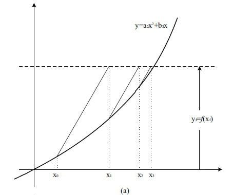
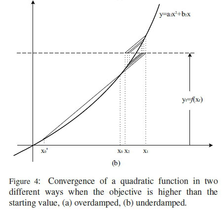
If the slope is reduced, a mixture of the overdamped and the underdamped response is found first. With further reduction, a complete underdamped case is found as shown in Fig. 4(b).

Lower Limit of m: The analysis is the same as the linear functions. For quadratic functions of can be written as,

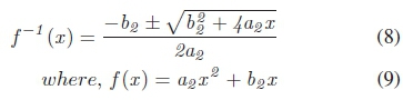
As the voltage magnitude can only be positive, the expression of (5) can be written as,

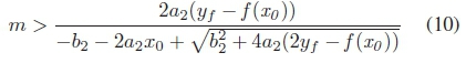
Any value of m above this value will make the system converging. The minimum value depends on yf ,x₀,a₂, and b₂. The value increases with the increase of yf. The relation between m, and xo is complicated. To avoid the complication, the slope at maximum possible xf is taken as the value of m that works for every xo. If xo is close to xf, it is the most efficient slope as analysed in Section 3.2. If not, the process operates in the overdamped case that is inefficient, but it is still better than calculating a new Jacobian for practical power systems as shown in Section 4.1. For the 118-bus system, one iteration of the WLS estimator takes around 42 times more time than the dishonest one, while around six iterations of dishonest method gains the same accuracy of the WLS method.

It is not expected that the starting point will always be lower than the target value; it may also be at a higher position. In case of x_f < x₀, the searching occurs in the downward slope. The two cases are shown in Fig. 5. The analysis is very much similar to the upward case, and a similar expression can be derived.

 

 

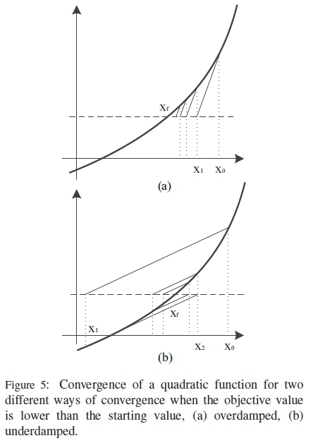
However, there has to be a single m irrespective of the position of x^f. The problem is resolved by taking the solution for the upward search. It is evident from the fact that for any , and x₀, if 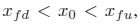. It can also be inferred that there will be only the overdamped case for the downward search with this value of m.

3.4 Sinusoidal Functions

Though the two typical cases can appear in sinusoidal operations, it is a bit complicated, as the slope of the function does not increase monotonically. The overdamped case is simple as shown in Fig. 6(a). In the underdamped case, if the slope at xi is less than m, the convergence cannot be ensured. So, (5) is applicable in a range of x where the slope is greater than m.

 

 

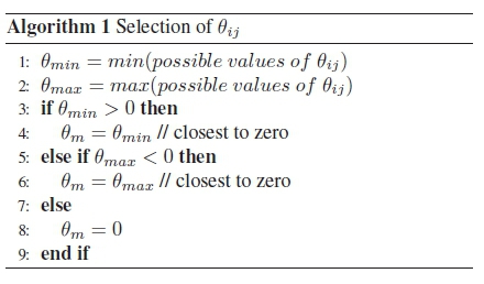
For power system, the phase angle of a bus with respect to the reference bus can vary a lot. Two connected buses usually keep a constant phase difference to maintain an expected real power flow between them. In case of typical faults, disturbances, or sudden load changes, the phase difference of the connected buses can change, but it usually does not exceed ±20°. In this short region, the sinusoidal function can be considered linear and the analysis for linear function can be applied. An easier choice is the maximum slope of this region that can ensure convergence. The maximum slope for a sine function occurs at θ = 0 and that for a cosine function occurs at . Due to the comparative values of a₃, and b₃, a value close to zero is preferred. However, taking the maximums slope can make it a slower process, and a better value can be obtained by choosing the closest possible value. For any transmission line ij, the angle corresponding to the maximum slope, θ_ηίcan be found with Algorithm 1.

 

 

4. MULTI-JACOBIAN METHOD

In the previous section, it is shown that the constant Jacobian calculated at the nominal values can fail with diverse states. On the other hand, a Jacobian with higher slopes can converge slower than the Jacobian with the nominal slope. A combined effort yields the proper solution.

4.1 Timing Profile of Constant Jacobians

To develop a comprehensive approach, it is important to have a practical view on the required time of the estimations using constant Jacobians. As mentioned earlier, the main advantages of the constant Jacobian methods come from the parallel implementation. So, the profiling is executed with parallel implementation on a GPU.

Setup ofthe Experiment: To test the dishonest method based state estimation, it is implemented on IEEE 118-bus test system with 186 transmission lines. Measurement errors are added artificially that vary in between 0.25-4% of the original values. The original values are collected under typical conditions of the states, i.e. |Ví | - 10, and θί - 0, for i = 2..N. For parallel estimation, an NVIDIA Tesla K20c GPU card with compute capability 3.5 is used. Based on the three steps, three different kernels are written that use different numbers of blocks and threads [20]. One of the major advantages of GPU is that it does not require any extra time to launch and finish a kernel. Therefore, the kernels can be executed sequentially without any delay [21]. The details of the GPU implementation can be found in [22].

For simulation, three sets of magnitudes are chosen to build the Jacobian matrix, |V_i| =0.9 pu, 1.0 pu, and 1.2 pu. For all cases, the angle is set according to Section 3.4. The required time is the product of the required number of iterations and the execution time of each iteration. The communication time is added with it. The trend of convergence of the WLS and the dishonest methods are shown in Fig. 7.

 

 

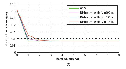
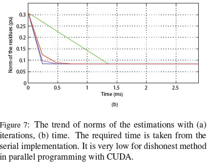
Analysis of the Results: It can be seen that the WLS method converges very close to the final value within only one iteration. On the other hand, the dishonest method with converges faster than other values of |V_i|. None of the dishonest methods take more than four iterations to achieve the same accuracy of one iteration of the WLS method.

However, due to the non-parallelisable part of the WLS estimator, one iteration of the WLS method takes around 2.7 ms while one iteration of the dishonest method takes around 64μβ. The communication time is around 26μs that is added to each measurement sample with multiple number of iterations. As a result, around 42 iterations of the dishonest method can run at the same time of one iteration of the WLS estimator. In serial implementation, around six iterations can run and the required time looks like Fig. 7(b).

4.2 Proposed Method

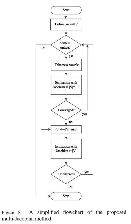
The proposed method is a simple addition to the existing method. From Fig. 7, it is clear that there exists a trade-off between the range and the speed of convergence for the dishonest method. The higher the slope, the bigger the range, and the slower the speed. As the power system rarely runs into any non-converging situation with nominal Jacobian, the main process runs with the existing method. Atthe same time, a few optional Jacobians are added in the process. The optional Jacobians are calculated with larger slopes (|V_i| = 1.2,1.4 etc.) and saved before starting the process. In case the nominal Jacobian fails, the options can be tried one by one as shown in Fig. 8. The number of options can be set with practical experiences.

 

 

5. ILLUSTRATIVE EXAMPLES OF FAILURE

It is already shown that a higher slope ensures convergence of the dishonest method. Though it is easy to derive the expression for the range of convergence for a single state, it is difficult for the multi-state case. However, the importance of the proposed method for the multi-state case can be realized through simulation.

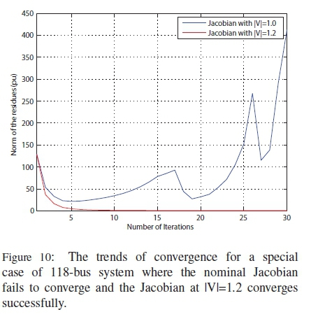
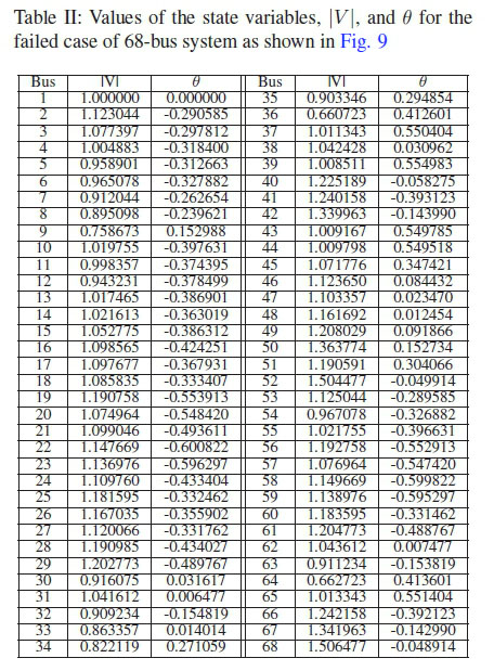
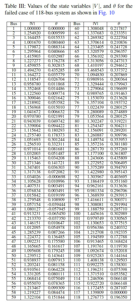
To show the case of failure, two Jacobians (at |V_i| =1.0 and at |V_i| = 1.2) are applied on IEEE 68, and IEEE 118-bus test systems operating under disturbances. The 68-bus system has 16 machines with 83 transmission lines. The details of the systems can be found in [23] (68-bus), and [24] (118-bus). The states for the failed cases are shown in Table II, and III of the Appendix. As the angles stay very close to zero, the nominal Jacobian is taken at the highest slopes at θ = 0. The voltage magnitudes vary a lot under the specified case.

The norms of the residues over the iterations of estimation are shown in Figs. 9, and 10. For both cases, it can be seen that the norms decrease in the beginning for both Jacobians. Then the nominal Jacobian (|V_i|= 1.0) starts a gradual increase after around ten iterations. It continues increasing and the process explodes eventually. On the other hand, the Jacobian with |V_i| = 1.2 converges with the iterations. These two examples clarify the importance of the proposed method.

 

 

 

 

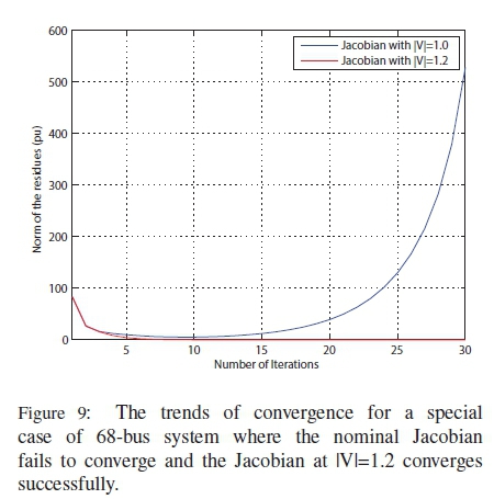
An important point to be noted that the norm can increase after a low value for |V_i|= 1.0. This means that a short distance with the starting value of the states, x₀ does not ensure convergence. The convergence depends on the closeness of the point of Jacobian and the point of operation.

As analysed in Section 3., the Jacobian should require higher |V_i| for higher variations of the voltage magnitudes of the buses. The minimum required |V_i|s are shown for different standard deviations of the magnitudes in Fig. 11.

 

 

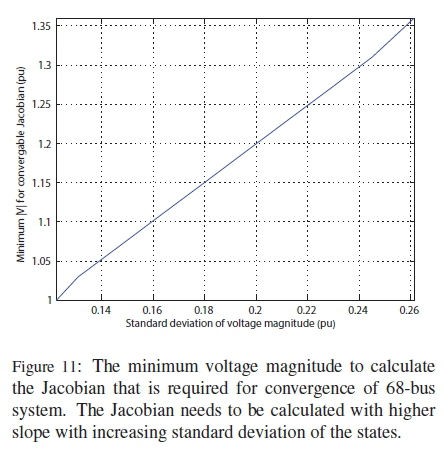
It can be seen that the nominal Jacobian fails for a standard deviation more than 0.1222. It is also observable that the minimum |V_i| keeps a linear relation with the standard deviation of the states.

It is important to remember that, the existing method with the Jacobian calculated at |V_i| = 1.0 that worked upto a variance of 0. 1222 is still a very strong tool. Because, under normal operating conditions, the variance usually does not exceed 0.05. Even with 10-20% load change of the 68-bus system, the magnitudes does not change much and they can be easily estimated. However, with very low probability, the states may reach some values that may not be possible to estimate using |V_i| = 1.0. Two such cases are shown in the Appendix. In one study, one out of 20000 samples failed to converge with |V_i| =1.0. Though the probability of such cases is low, it can be crucial as the states may undergo very high change during that time. Under these failed cases, the safer choice will be to calculate the Jacobian with a higher value of |V_i|, not with a lower one.

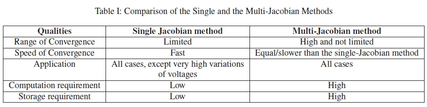
The single and the multi-Jacobian methods are compared in Table I. The range of convergence refers to the maximum variation of the states with which the method can converge. The speed of convergence is the inverse of the time required to converge. The computational requirement is shown for the case where both methods converge. The storage requirement denotes the memory needed for saving the M-matrices for different |V_i|.

 

6. CONCLUSIONS

A special issue of convergence for the traditional constant Jacobian based estimator for power systems has been addressed in this study. It is shown that the Jacobian calculated with the nominal values of the states may fail under special circumstances. The problem can easily be solved using an alternative Jacobian taken at a higher slope. To keep both the speed and the reliability of the estimator, a multi-Jacobian method is also proposed. The issue of convergence for large variations of the states needs to be investigated for all computational processes of power systems where the Jacobian is kept constant like the stability analysis or the optimal power flow. The analysis requires further research to explore the possibility of a complete expression of convergence for the multi-state case. It will help us to find more loopholes in the processes of the constant Jacobian.

 

7. ACKNOWLEDGEMENT

This work is supported in part by the US National Science Foundation (NSF) under grant #1312260, #1408141 and the Duke Energy Distinguished Professor Endowment Fund. Any opinions, findings and conclusions or recommendations expressed in this material are those of the author(s) and do not necessarily reflect the views of NSF or Duke Energy Foundation.

 

REFERENCES

[1] W. Li and L. Vanfretti, "A PMU-based state estimator considering classic HVDC links under different control modes," Sustainable Energy, Grids and Networks, vol. 2, pp. 69-82, 2015.         [ Links ]

[2] F. F. Wu, "Power system state estimation: a survey," International Journal of Electrical Power & Energy Systems, vol. 12, no. 2, pp. 80-87, 1990.         [ Links ]

[3] A. Abur and A. Exposito, Power System State Estimation: Theory and Implementation. New York, NY: Marcel Dekker Inc., 2004.         [ Links ]

[4] N. Xia, H. B. Gooi, S. Chen, and M. Wang, "Redundancy based PMU placement in state estimation," Sustainable Energy, Grids and Networks, vol. 2, pp. 23-31,2015.         [ Links ]

[5] B. Otto, Linear Algebra with Applications. Upper Saddle River, NJ: Prentice Hall, 2005.         [ Links ]

[6] F. C. Schweppe and J. Wildes, "Power system static-state estimation, Part I: Exact model," IEEE Trans. Power Apparatus and Systems, vol. PAS-89, no. 1, pp. 120-125, Jan. 1970.         [ Links ]

[7] F. C. Schweppe and D. B. Rom, "Power system static-state estimation, Part II: Approximate model," IEEE Trans. Power Apparatus and Systems, vol. PAS-89, no. 1, pp. 125-130, Jan. 1970.         [ Links ]

[8] V. Miranda, D. Srinivasan, and L. M. Proenca, "Evolutionary computation in power systems," International Journal of Electrical Power & Energy Systems, vol. 20, no. 2, pp. 89-98, 1998.         [ Links ]

[9] J. Carpentier, "Optimal power flows," International Journal of Electrical Power & Energy Systems, vol. 1, no. 1, pp. 3-15, 1979.         [ Links ]

[10] D. Alves, L. Da Silva, C. Castro, and V. da Costa, "Parameterized fast decoupled power flow methods for obtaining the maximum loading point of power systems: Part I. Mathematical Modeling," Electric Power Systems Research, vol. 69, no. 1, pp. 93-104, 2004.         [ Links ]

[11] A. Monticelli, State estimation in electric power systems: A generalized approach. Norwell, MA: Kluwer Academic Publishers, 1999.         [ Links ]

[12] S. K. Khaitan and J. D. McCalley, "SCALE: A hybrid MPI and multithreading based work stealing approach for massive contingency analysis in power systems," Electric Power Systems Research, vol. 114, pp. 118-125, 2014.         [ Links ]

[13] S. Jankovic and B. Ivanovic, "Application of combined Newton-Raphson method to large load flow models," Electric Power Systems Research, vol. 127, pp. 134-140, 2015.         [ Links ]

[14] E. Lindholm, J. Nickolls, S. Oberman, and J. Montrym, "NVIDIA tesla: A unified graphics and computing architecture," IEEE Micro, vol. 28, no. 2, pp. 39-55, Mar. 2008.         [ Links ]

[15] K. A. Clements, "Observability methods and optimal meter placement," International Journal of Electrical Power & Energy Systems, vol. 12, no. 2, pp. 88-93, 1990.         [ Links ]

[16] S. Soliman and M. El-Hawary, "Measurement of power systems voltage and flicker levels for power quality analysis: a static LAV state estimation based algorithm," International Journal of Electrical Power & Energy Systems, vol. 22, no. 6, pp. 447-150, 2000.         [ Links ]

[17] P. Rousseaux, T. Van Cutsem, and T. D. Liacco, "Whither dynamic state estimation?" International Journal of Electrical Power & Energy Systems, vol. 12, no. 2, pp. 104-116, 1990.         [ Links ]

[18] T. Bi, X. Qin, and Q. Yang, "A novel hybrid state estimator for including synchronized phasor measurements," Electric Power Systems Research, vol. 78, no. 8, pp. 1343-1352, 2008.         [ Links ]

[19] A. A. da Silva and V. Quintana, "Pattern analysis in power system state estimation," International Journal of Electrical Power & Energy Systems, vol. 17, no. 1, pp. 51-60, 1995.         [ Links ]

[20] J. Nickolls, I. Buck, M. Garland, and K. Skadron, "Scalable parallel programming with CUDA," Queue, vol. 6, no. 2, pp. 40-53, Mar. 2008.         [ Links ]

[21] J. Nickolls and W. J. Dally, "The GPU computing era," IEEE Micro, vol. 30, no. 2, pp. 56-69, Mar. 2010.         [ Links ]

[22] M. A. Rahman and G. K. Venayagamoorthy, "Dishonest Gauss Newton method based power system state estimation on a GPU," in Proc. Clemson University Power Systems Conference (PSC), Clemson, SC, USA, Mar. 2016, pp. 1-6.

[23] B. Chaudhuri, R. Majumder, and B. C. Pal, "Wide-area measurement-based stabilizing control of power system considering signal transmission delay," IEEE Trans. Power Systems, vol. 19, no. 4, pp. 1971-1979, Nov 2004.         [ Links ]

[24] R. D. Zimmerman, C. E. Murillo-Sánchez, and D. Gan, "Matpower," PSERC.[Online]. Software Available at: http://www.pserc.cornell.edu/matpower, 1997.

 

 

APPENDIX