


Services on Demand
Article
 English (pdf)
 Article in xml format
 Article references
Indicators

Related links
-
 Cited by Google
 -
 Similars in Google
Share

 Permalink
Water SA
On-line version ISSN 1816-7950
Print version ISSN 0378-4738
Water SA vol.50 n.1 Pretoria Jan. 2024
http://dx.doi.org/10.17159/wsa/2024.v50.i1.4022
RESEARCH PAPER
Improved flood quantile estimation for South Africa
D van der Spuy; JA du Plessis
Department of Civil Engineering, Stellenbosch University, P/BagXl, Matieland 7602, South Africa
ABSTRACT
The performance of the most frequently used flood frequency probability distributions in South AfriCd (Log-Normal, Log Pearson3 and Generalised Extreme Value) were reviewed and all tend to perform poorly when lower exceedance probability frequency events are estimated, especially where outliers are present in the dataset. This can be attributed to the challenge when analysing very limited 'samples' of annual flood peak populations, which are an unknown. At present outliers are inadequately 'managed' by attempting to 'normalise'the flood peak dataset, which conceals the significance of the observed data. Thus, to adequately consider the outliers, this study was undertaken with the aim to improve the current statistical approach by developing a more stable and consistent methodology to estimate flood quantiles. The approach followed in the development of the new methodology, called IPZA, might be considered as unconventional, given that a multiple regression approach was used to accommodate the strongly skewed data, which are often associated with annual flood peak series. The main advantages of IPZA are consistency, the simplicity of application (only one set of frequency factors for every parameter, regardless of the skewness),the integrated handling of outliers and the use of conventional method of moments, thereby eliminating the need to adjust any moments. The performance of IPZA exceeded initial expectations. The results are more consistent ind, by taking outliers into account, appear to be more sensible than existing probability distributions. It is recommended that IPZA should be used as a valuable addition to the existing set of decision-making tools for hydrologists/engineers performing flood frequency analyses.
Keywords: flood, quantile, frequency, probability, exceedance, distribution, practical
INTRODUCTION
Floods rank among the topmost devasting natural disasters. The 1931 Yangtze (Yangzi) River flood in Southern China, is indisputably still considered the worst natural disaster of the 20lh century. The flood inundated 180 000 km2 and an estimated 3.7 million people lost their lives (Courtney, 2018) -however, one should be aware that figures relating to damages and deaths are estimates and may vary from reference to reference. In South Africa (SA) the floods of 1981,1984,1987,1988 and more recently 2000 immediately come to mind. The flood in the Buffels River in 1981, which inundated the town of Laingsburg, caused 90 people to lose their lives and caused damage in excess of 10 million ZAR (1981 values), was caused by what is popularly referred to as a Black South-Easter weather situation (Roberts and Alexander, 1982). Although Domoina in 1984 is commonly referred to as a tropical cyclone, it only officially reached the status of a severe tropical storm. Domoina caused widespread flooding in northern KwaZulu-Natal (KZN) in SA, Mozambique (Moz) and eSwatini, causing widespread damage to road infrastructure and property of more than 100 million ZAR (1984 values) and over 200 reported deaths in South Africa alone (Kovács et al., 1985). The main cause of the 1987 floods in the southern part of KZN was an intense off-shore cut-off low pressure system. The damage was calculated to have been amongst the most devasting that has occurred in SA. Damage to property, agriculture (including several hundred farm dams that were breached), communications and infrastructure amounted to approximately 400 million ZAR, with 388 reported deaths and 150 000 people left homeless (Van Bladeren and Burger, 1989). During two periods in February 2000, tropical weather systems, which included the tropical cyclone Eline, making landfall at the Moz coast in the Beira area, resulted in extreme rainfall leading to devastating floods. The excessive financial impact of approximately 1.5 billion ZAR (2000 values) to infrastructure and water services in SA, as well as social impact (at least 600 people in Moz lost their lives and hundreds of thousands of people were displaced) was most probably the worst experienced in living memory in Southern Africa (Dyson and Van Heerden, 2001).
These extreme events occur in relatively short annual maximum series (AMS) flood peak record lengths, which engineers and hydrologists use to perform flood frequency analyses (FFAs). These analyses are used to determine design floods for dams and bridges, for example, as well as to determine flood lines along rivers, optimal time frames for construction, inundation of vulnerable crops, etc.
In flood hydrology the benefit of having an entire population of AMS of flood peak records, to test the AMS sample records against, does not exist. From very short AMS samples, hydrologists have to estimate the underlying probability distribution of the AMS population. It is thus of extreme importance to constantly strive to improve the tools available to engineers and hydrologists, to increase the confidence in FFA.
Existing probability distributions commonly applied in South Africa
The probability distributions most used in SA for FFA are the Log-Normal (LN), Log-Pearson Type III (LP3) and the Generalised Extreme Value (GEV) distributions (Alexander, 1990; SANRAL, 2013; Van der Spuy and Du Plessis, 2022a). Both the LP3 and GEV distributions have provided good results (DWS, 1993-2021) and the practice is to apply both and use the one that seems to fit the observed data best. Van der Spuy and Du Plessis (2022a) illustrated that all of the distributions lack consistency, which is mainly caused by the inability to deal properly with outliers in an AMS of flood peak data. They showed that, although the GEV proved to be insensitive to low outliers, all distributions are susceptible to high outliers. Ball et al. (2019) consider outliers as observations that are inconsistent with the general trend of the rest of the data. Frost (2019) stated that, while there is no strict statistical rule or mathematical definition to identify outliers, guidelines exist through which possible outliers can be identified. The Zscore (one such guideline) also provides a measure to compare relative probabilities associated with relative magnitudes of the data. Since nearly 100% of the data will be within 3 standard deviations of the mean, data with a Z-score higher than 3, or lower than -3, can be outliers (Brownlee, 2018; Frost, 2019). Van der Spuy and Du Plessis (2022a) expressed the need for a probability distribution which will provide more consistent flood frequency estimations. They also proposed that the plotting position (PP) approach should be improved, especially concerning outliers. Van der Spuy and Du Plessis (2022b) developed an alternative PP technique, the Z-set PP. The Z-set PP offers an improved and more realistic representation of outliers, with a further advantage of being less susceptible to different record lengths than the existing PP techniques. The Z-set PP was considered as an essential tool to the flood frequency analyst to assist in more consistent choices of appropriate probability distributions.
Purpose of study
The purpose of this study was to develop a more consistent methodology to estimate flood quantiles (discharges with specified probabilities of exceedance) that would not be as sensitive to outliers as the most frequently used flood frequency probability distributions in South Africa. Consequently, the Z-set PP formed an integral part in the study.
The sensitivity to outliers of the developed methodology will be evaluated against that of the LP3 and GEV
METHODOLOGY
Statistics were identified, computed from the AMS data at selected flow gauging sites (referred to as sites henceforth), which could be considered as potential parameters of the 'underlying probability distribution, in an FFA. The study was performed in three phases to find the most appropriate statistics that would be used as parameters for a new flood quantile methodology
Phase 1: Evaluation of statistics as potential independent variables
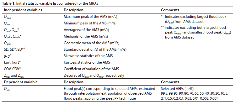
Multiple regression analyses (MRAs) were used to determine which of the identified potential statistics have little or no impact on the development of a new flood quantile methodology. For the MRAs the following variables were identified (detailed in Table 1):
• As independent variables - the identified potential statistics were considered
• As dependent variables - flood peak values, referred to as Observed' floodpeaks (Qobs) at identified annual exceedance probabilities (AEPs), were used
Values for Qobs were estimated for the identified AEPs by interpolation and extrapolation of the floodfrequency relationship between the AEPs (applying the Z-set PP) and the observed AMS flood peaks (estimated from observed (recorded) stage levels).
In this phase of the study MRAs were conducted for every identified AEP to estimate a flood peak (Qest) that could be compared graphically, corroborated by the coefficient of determination (R2), to the corresponding Qobs. for every flow site.
The identified variables, which did not contribute to improve the results in any way, were eliminated
Phase 2: Identify parameters for flood quantile model
Using an MRA-approach, various clusters (henceforth used in referring to combinations of the remaining independent variables) were assessed to estimate the dependent variables (Qobs).
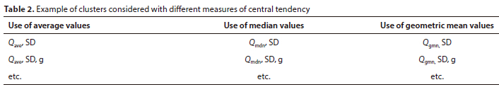
Due to the parameters used in most existing probability distributions, it was anticipated that a cluster with one of the measures of central tendency as integral part, accompanied by the SD and g, would result in the most likely solution to the study Consequently, Table 2 depicts examples of clusters that were considered and assessed.
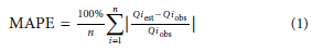
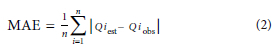
For every cluster at every site, MRAs were conducted at all selected AEPs to estimate values of Qest. Instead of just graphically comparing Qest with the corresponding Qobs, key performance indicators (KPIs) were used to rank the relative performance of the different clusters. All these KPIs perform differently, mainly related to the magnitude of the values involved - therefore, two KPIs were chosen, namely, the mean absolute percentage error (MAPE) and the mean absolute error (MAE) depicted in Eq. 1 and Eq. 2, respectively. The MAE is likely to suggest relatively large errors' at lower AEPs (large flood peaks), while the percentage difference might be very small; on the other hand, MAPE might suggest large percentage errors' at higher AEPs, while the absolute errors (in terms of flood peaks) could be insignificant in relation to flood hydrology. Therefore, these tests were considered as relative assessments of performance, rather than absolute, for the purpose of this study
In FFA the 'design flood' range is of more practical value than for the AEP range > 50%. Thus, MAPE and MAE were considered more applicable, respectively, for AEP range < 50% and AEP range > 50%.
and
where:
MAPE = mean absolute percentage error (%)
MAE = mean absolute error (m3/s)
n = sample size = number of AEP values used for AEP< 50% and AEP range > 50% ranges
Qiobs = observed flood peak related to an AEP at observation 'i' (m3/s)
Qiest = estimated flood peak related to an AEP at observation 'i' (m3/s)
From these results the cluster that provided the best fit, on average, to the observed AMS flood peaks was used to develop a flood quantile model.
Phase 3: Flood quantile model
Wheeler (2022) expressed his concern that many believe the first step in data analysis is to check for normality. If the data are strongly skewed, as is often the case with the AMS of flood peaks, Wheeler explained that it is a "mathematical fact of life" that no skewed probability model exists to fit these data. Wheeler (2009) also stated that if data are transformed to make them appear to be 'more normal', it is likely to "endup with a beautiful, but completely incorrect, analysis". As a practical alternative, the MRA results of the chosen cluster were used to find an empirical solution for the flood quantile model. Consequently, the independent variables were used as the parameters for the flood quantile model, while the regression coefficients, associated with the AEPs, correspond to the frequency factors. However, given that the wide range of AEPs did not provide sensible independent variables, an associated standardised variable was considered. Two standardised variables were considered, namely, the standardised variate used for the log-normal distribution (WT) and the standardised variate for the EVI distribution (Wp). Both are considered to be suitable, but the standardised variate Wp was chosen, merely because of the simplicity of its equation.
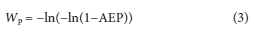
To estimate continuous frequency factors, at different AEPs used in the study, polynomial functions were used. For each statistical parameter the regression coefficients, determined for every AEP, were considered to be the dependent variables (y), while the associated standard variate Wp was considered to be the independent variable (x).
The general form of the polynomial function (using Wp) is:

where:
Kp = frequency factor
M = denotes the degree of the polynomial (determined by optimum correlation coefficient)
am = coefficient of the mth degree term
The general form of the flood quantile model can be written as:
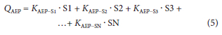
where:
Qaep = flood peak associated with an AEP (m3/s)
Si = ithstatistical parameter, for i from 1 to N
Kaep-si = frequency factor, related to AEP for Si
N = total number of statistics considered
DATA
Similar to the study by Van der Spuy and Du Plessis (2022b), only AMS flood peak data were considered in this study. It has been reported that the partial duration series (PDS) flood peak data approach does not really improve results, especially for an ARI (annual recurrence interval) higher than 10 years (Mkhandi et al, 2005; Karim et al, 2017). Srikanthan (2014) also concluded that, since the AMS results in the smallest bias in most cases, the use of AMS in FFA is preferred to PDS.
Data sources
Van der Spuy and Du Plessis (2022b) used 18 sites for their study A further 23 sites were added to these sites for this study, ensuring more comprehensive coverage across South Africa. The objective was to find suitable sites, with verified reliable data, in areas and drainage regions not covered previously. There was an attempt to keep the record lengths at 60 years and above; however, 2 sites had record lengths of 58 and 57 years, respectively, and 1 site a record length of only 39 years. These sites were included to provide some data in areas where appropriate sites are very limited.
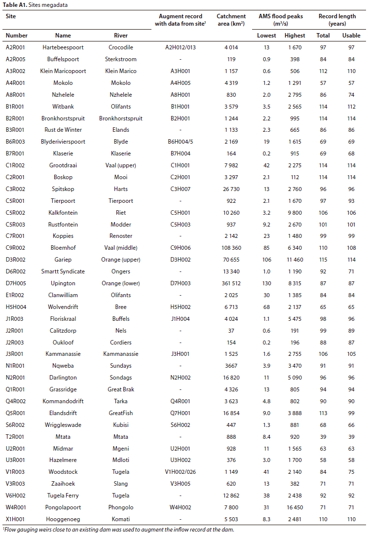
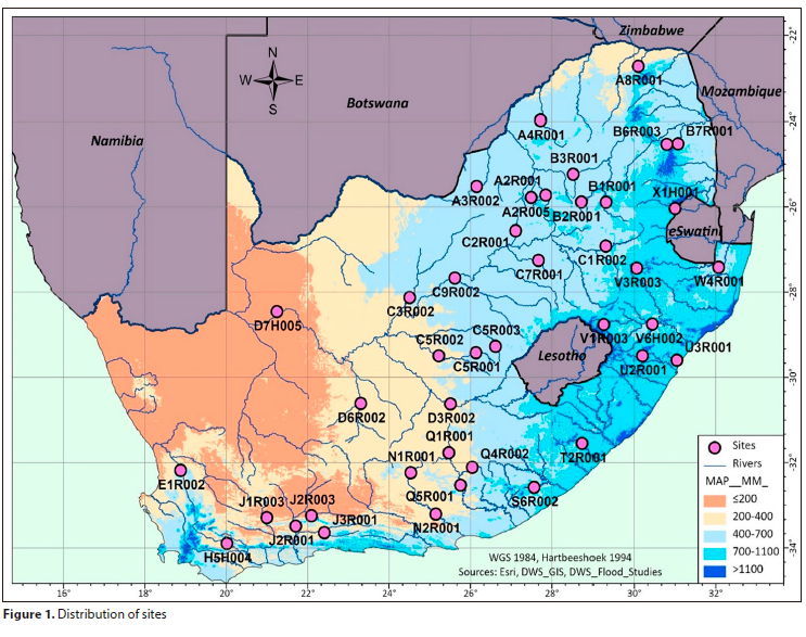
The location of the selected 41 flow sites is depicted in Fig. 1. Relevant metadata for the flow sites, which include 37 dam and 4 gauging weir sites with a combined database of 3 615 years of usable AMS flood peaks, are provided in Table A1 (Appendix) The sites amply cover the vast diversity of meteorological and hydrological conditions experienced across SA.
Extracted data used in study
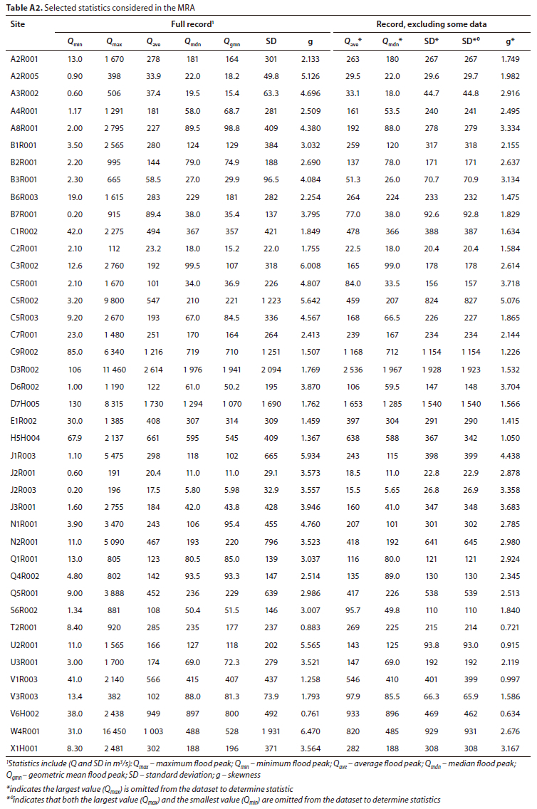
Selected statistics computed from the AMS at each site, utilised as independent variables in the MRA approach, are presented in Table A2 (Appendix). The most appropriate statistics, from these selected statistics, constitute the input into a probability model to produce estimated flood peak values (Qest) at corresponding AEPs.
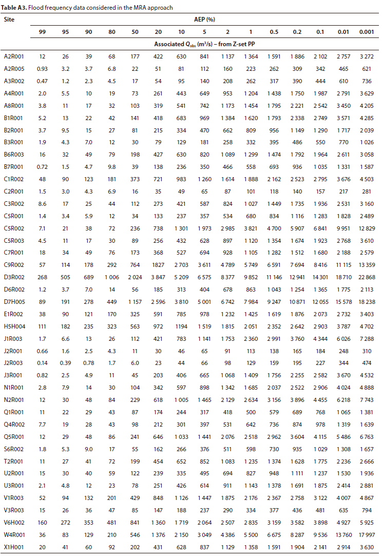
Selected flood frequency data (Qobs vs selected AEPs), applied as dependent variables in the MRA, are presented in Table A3 (Appendix).
RESULTS
The results are presented below in sections corresponding to the phases defined in the methodology. The acronym of the proposed flood quantile model is identified in advance, since it appears on figures presented as part of the results and is defined as the IPZA (Improved Probability-model, South Africa).
Phase 1: Evaluation of statistics as potential independent variables
MRA clusters, containing numerous combinations of the initially selected statistics (Qmax, Qmin, Qave, Qmdn, Qmdn*, Qgmn, SD, SD*, SD*°, g, g*, COV, COV*, COV*0, Zmax and Zmin), were performed and assessed. As could be expected, variables such as Qave, Qmdn, Qgmn and SD were considered as potentially significant. Unexpectedly, and contrary to existing practice and beliefs, the initial evaluations suggested that the effect of including skewness (g) might be statistically insignificant. It was thus hypothesised that omitting g would either have no effect or potentially improve the results. Since the SD relates to the slope of the relative distribution of the data points (in this case a scatterplot of flood peaks against their corresponding Zscores), and is thus affected by outliers, it was furthermore hypothesised that replacing g with SD* might improve the outcome. In addition, SD*, SD*° and SD** were also considered as being potentially significant. The example in Fig. 2 (from an MRA at a chosen AEP) illustrates what led to the suggestion that replacing g with SD* might improve results.
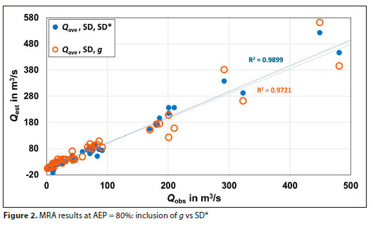
Several clusters were evaluated graphically, corroborated by the coefficient of determination (R2), to determine whether they could contribute to improve the results, or not (also illustrated by Fig. 2). After much experimentation and evaluation, the following statistics/parameters were excluded (Qmax, Qmin, Zmax, Zmn, Qave*, Qmdn*, g*> kurt, kurt*, COV, GOV*) and the following retained (Qave,. Qmdn, Qgmn, SD, SD*,g) for more detailed analyses.
Phase 2: Identify parameters for flood quantile model
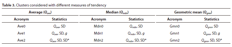
To find the best grouping of parameters, different clusters were used with one of the measures of central tendency as the integral statistic, supplemented by SD and g.
To test the hypothesis that replacing g with SD* may improve results, clusters were added where g was replaced by SD*. The clusters considered and the selected statistics are depicted in Table 3.
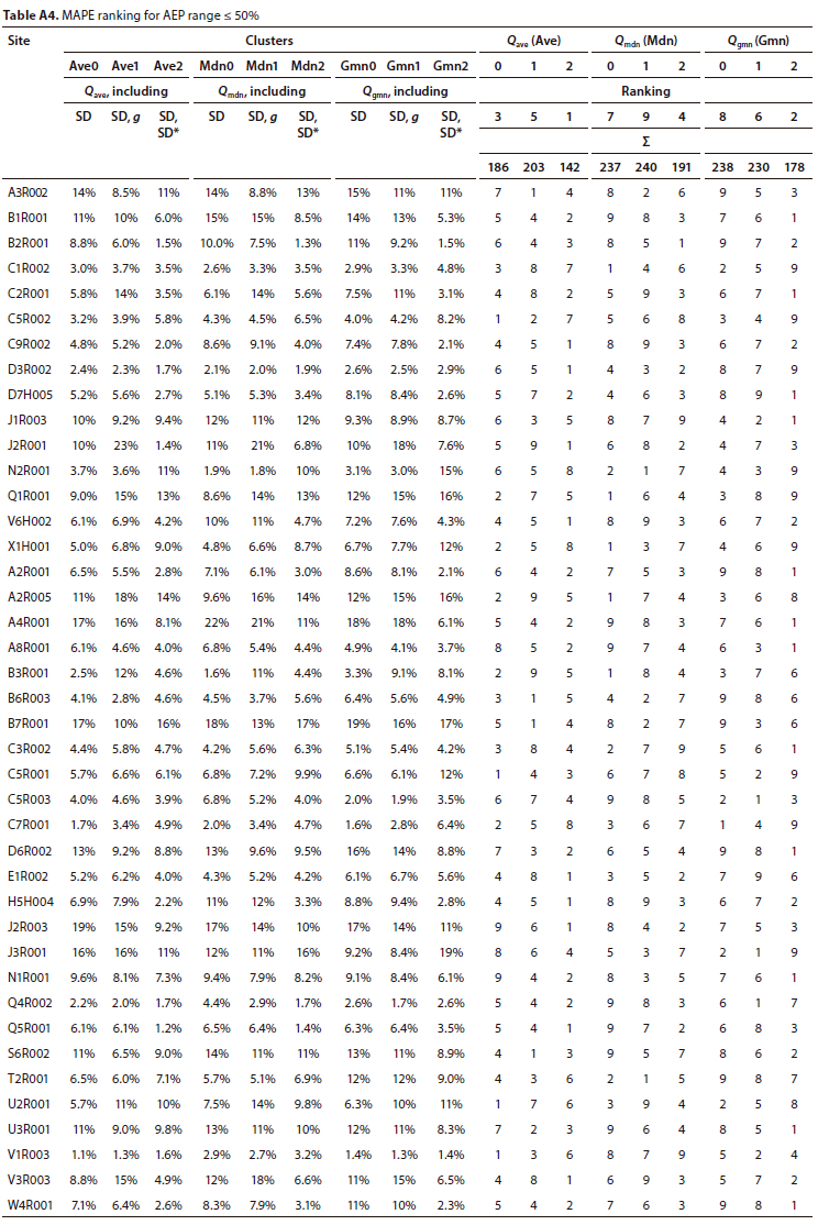
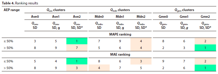
MRAs were conducted at all stations for all selected AEPs for every cluster (a total of 198 MRAs). The summarised outcome of the ranking results of the MAPE and MAE KPIs, based on the average value for an AEP range at all stations, is presented in Table 4 -the MAPE results for the AEP < 50% range are provided in Table A4 (Appendix).
Based on the ranking results, bearing in mind that the MAPE is considered to be more relevant for AEPs < 50% and the MAE for AEPs > 50%, the following was noted:
• As hypothesised, regardless of the measure of tendency used, the clusters with the g statistic generally performed the worst - the exception being Gmnl for AEPs < 50%.
• Regardless of the measure of central tendency used, the clusters with the SD* statistic performed the best overall - the exception being MdnO for AEPs > 50% (only with MAE).
• The poor performance of the Qmdn clusters was disappointing since the median (as with the geometric mean) is generally considered to be closer to the estimated 50% AMS flood peak (ξ to a 2-year ARI).
For AEPs < 50% both MAPE and MAE indicated that Cluster Ave2 (Qavc SD and SD*) performed the best - with Cluster Gmn2 being 2nd best.
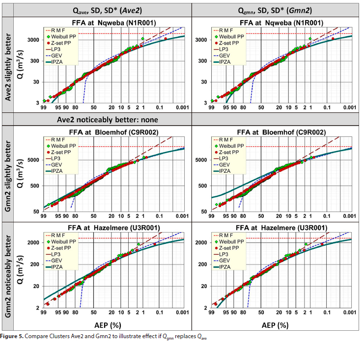
For AEPs > 50% (ARI < 2 years) both MAPE and MAE indicated that Cluster Gmn2 (Qgmn SD and SD*) performed the best.
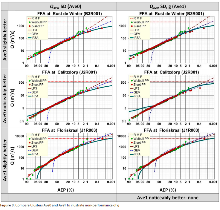
To illustrate some of the above findings, visual comparisons of clusters are presented, indicating which cluster is categorised as noticeably better or only slightly better, than the other. For each category the sites, which indicate the most noticeable difference between the clusters, were selected to illustrate the differences and are depicted below, as follows:
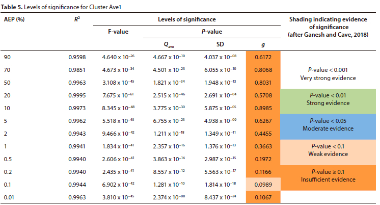
• The suggestion, that the g-statistic is not a statistically significant variable, is visually illustrated in Fig. 3 (AveO vs Avel), supported by the estimated significance levels, at selected AEPs in Table 5.
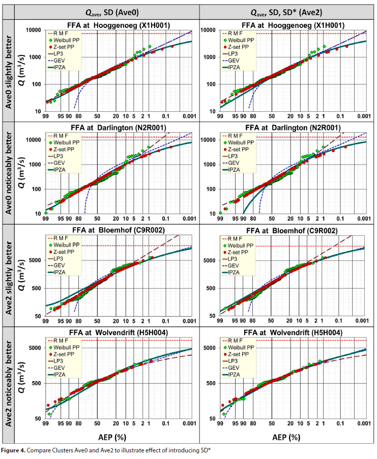
• 'Ihe effect of introducing the SD* statistic is illustrated in Fig. 4 (Ave0 vs Ave2).
• The effect of replacing Qave with Q is illustrated in Fig. 5 (Ave2 vs Gmn2).
• In all ensuing figures, flood quantile plots are fitted using method of moments.
• The estimated RMF (regional maximum flood; after Kovács, 1988) is also depicted on the relevant figures.
Combining the results of Ave2 (for AEPs < 50%) and Gmn2 (for AEPs > 50%) was considered; however, this created a discontinuous transition in the region where the AEP = 50%.
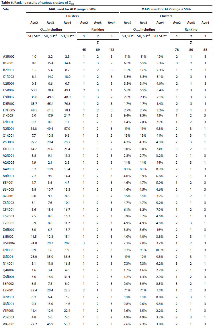
To confirm that Cluster Ave2 might not be further improved, by inadvertently excluding more pertinent statistics, it was compared with Cluster Ave3 (Qave, SD, SD*°) and Cluster Ave4 (Qave, SD, SD**) and the results are presented in Table 6, where the MAE was used in the AEP range > 50% and MAPE was used in the AEP range < 50%. SD*° was calculated by excluding the highest and lowest flood peaks from the AMS dataset and SD** was calculated by excluding the highest 2 flood peaks from the AMS dataset.
The final choice was primarily guided by the relevance of the results in the design flood range, as well as avoiding unnecessarily complicated solutions. Accordingly, Ave2 was selected as the best cluster.
Phase 3: Flood quantile model
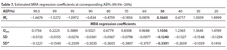
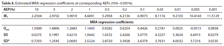
Estimated regression coefficients, for the independent variables used in the MRAs of Cluster Ave2, are provided in Table 7 and Table 8, for every chosen AEP with the associated standardised variate Wp.
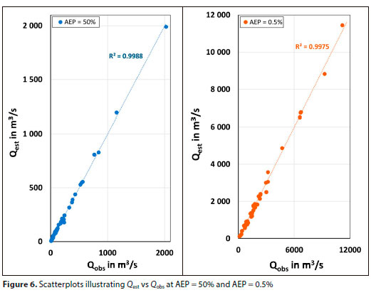
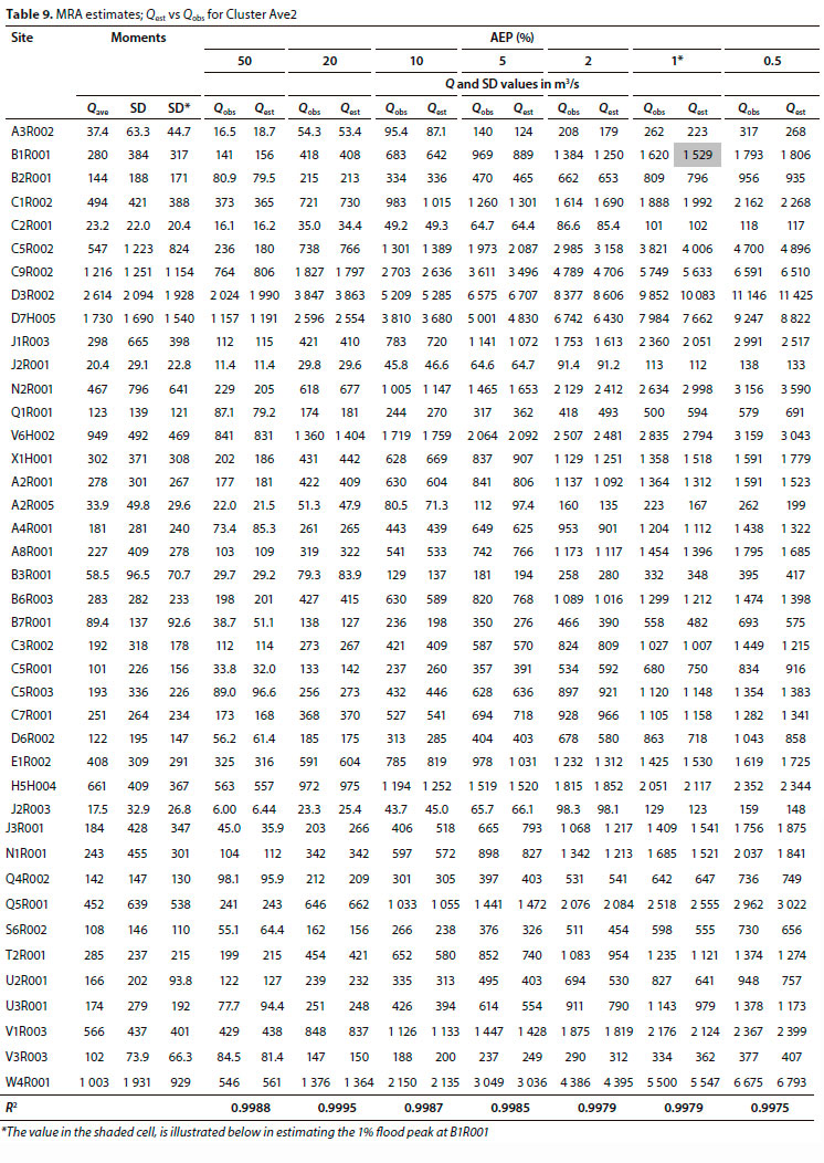
To limit the size of the tables presented, only the most common AEPs < 50% are included. A comparison of Qobs with Qest results, from MRA for Cluster Ave2, is provided in Table 9, with illustrative scatterplots in Fig. 6.
To illustrate the estimation of the 1% flood peak at B1R001:
Relevant statistics for B1R001: Qave = 280 m7s, SD = 384 m3/s and SD* = 317 m3/s (Table A2) • At AEP = 1%: the respective regression coefficients are 1.1443, 1.0642 and 2.5224 (Table 8)
• Therefore, Qest = 1.1443 · 280 + 1.0642 · 384 + 2.5224 · 317 = 1 528.66 m7s
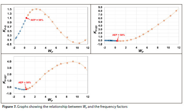
The regression coefficients become the frequency factors and a polynomial function (Eq. 4) was fitted to establish a continuous relationship between the frequency factors and Wp to estimate intermediate values. The graphs, showing the relationships between Wr and the estimated frequency factors KP_Q, KP_SD and Kp sl), respectively associated with Qave, SD and SD*, are provided in Fig. 7.
From the selected Ave2 cluster, the parameters for the flood quantile model are Q.ave, SD and SD*. Equation 5 can thus be rephrased as the general form of the IPZA flood quantile equation:
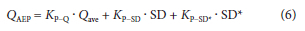
where: Kp_Q, KP_SD and -KP_SD, are the frequency factors for their respective parameters.
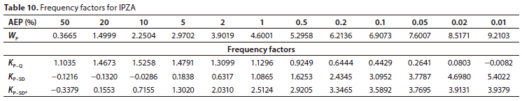
The estimated frequency factors for selected AEP values are provided in Table 10.
Assessment of IPZA
In this section a brief assessment is done on the tendency of IPZA to under- or overestimate, and on the performance of IPZA in relation to outliers.
Under- or overestimation
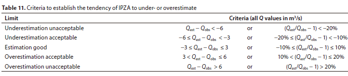
It is beneficial to identify whether a particular probability distribution or flood quantile model tends to overestimate or underestimate. Applicable criteria are not readily available and appear to depend on the focus of the study. Haddad and Rahman (2012), considering the focus for their study, suggested that a Qcsl/Qob, ratio value of between 0.5 and 2 may be considered as acceptable. However, an underestimation of 50% and overestimation of 100% is considered completely unacceptable for this study and the suggested criteria in Table 11 were utilised to determine whether IPZA tends to underestimate or overestimate, and whether it was considered acceptable or not.
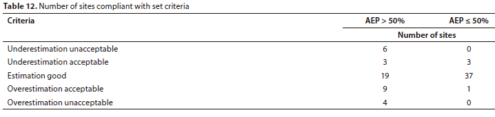
The criteria were applied to all sites at every AEP and the average outcome was calculated for every site separately for the AEPs > 50% and the AEPs < 50%. The number of sites compliant with the criteria is depicted in Table 12.
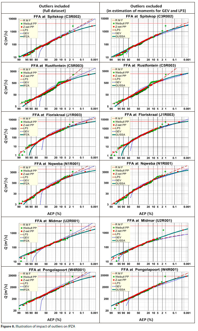
In the design flood range IPZA performs very well using the defined criteria. For AEP > 50% the performance is slightly lower, but it still outperforms the GEV in this range (refer to Fig. 3 to Fig. 5, as well as Fig. 8).
Outliers
The performance of IPZA, in relation to how it is affected by outliers, will be pivotal in whether its performance is an improvement to existing probability distributions used in South Africa or not. The study sites with the most distinctive outliers are depicted in Fig. 8 as an illustration.
It is important to note in Fig. 8 that:
• The PPs represent the full AMS for both columns (outlier still part of the AMS)
• The outlier was removed in the estimation of the moments for GEV and LP3 to assess if it would fit the rest of the data better (IPZA was developed to accommodate outliers -there is no need to remove it)
From Fig. 8 it is evident that the GEV and LP 3 probability distributions, with the outlier excluded in the estimation of moments, plot much closer to IPZA, especially in the case of the GEV - the exception being the Midmar Dam, where PILFs (potential influential low flows) can severely influence the LP3.
DISCUSSION
The primary objective of this study was to propose a more consistent flood quantile methodology. The Z-set PP established the foundation for the development of the proposed IPZA flood quantile model. Although only 41 sites were used in the study, due to record length and data accuracy constraints, the coverage of sites across South Africa and the diversity of meteorological and hydrological conditions were well covered.
The study leading to the culmination of the IPZA flood quantile model, has unveiled some noteworthy observations:
• Wheeler (2022) expressed his concern that many believe the first step in data analysis is to check for normality. With IPZA there is no need to transform data or moments to make the distribution 'more normal', which makes it simple to use.
• Wheeler (2022) also explained that no skewed probability model exists to fit strongly skewed data. To use the MRA approach to estimate parameters for a flood quantile model might perhaps be considered as unconventional, but the results proved to be exceptionally good.
• The hypothesis that to omit g would either have no effect or improve the results was proved correct. This might seem to be a surprising result, but it could have been expected, considering the statement by Wheeler (2011) that to estimate g with a similar degree of confidence than the location statistics (Qave and SD), 6 times the record length is required. This might be the reason why some distributions often do not perform well, considering that the sample g is most probably not representative of the skewness of the underlying distribution.
• The hypothesis that the addition of SD* might improve results, was also proved correct. It appears that SD* might compensate for the instances where SD is affected by extremely high flood peaks, resulting in an inaccurate slope for the relative distribution of data points. Where no outlier is present SD * SD*, with no effect on results, as illustrated in Fig. 4 at Wolvendfrift and Bloemhof Dam.
• Wide-ranging speculation about whether the median statistic should be used instead of the average, was challenged by the outcome of this study, demonstrating the average value to be the best option (even the geometric mean proved to be a more viable option than the median).
• The IPZA seems to be virtually unaffected by outliers. Consequently, the problem to decide whether to ignore a suspected outlier, or not, should no longer be a concern.
• The IPZA is extremely consistent in the design flood range (AEP < 50%; ARI > 2 years) in estimating flood peak frequencies from AMS. According to the set criteria, the estimated flood peaks are considered as 'good' at 37 of the 41 sites - and 'acceptable' at the remaining sites.
CONCLUSION
The Z-set PP, which adjusted the PP of outliers, provided the basis for finding a corresponding solution for a more consistent flood quantile methodology. Whether the IPZA can be considered as bounded, or not, is inconclusive at this stage. However, from the results presented it can be concluded that the IPZA is probably more likely to have an upper bound than the GEV or LP3.
The IPZA seems to be much more stable and consistent in the estimation of flood quantiles, compared to the GEV and the LP3, as depicted on all the included FFA results.
Further research to improve the IPZA should include:
• Investigate the less satisfactory estimates for AEPs > 50%.
• The performance of IPZA should be evaluated with shorter AMS record lengths, at sites with good, verified data.
• Although the study sites did cover diverse meteorological and hydrological conditions, it should be tested with datasets from outside South Africa to further evaluate its performance.
It is recommended that the IPZA be used as a valuable addition to the existing set of decision-making tools for flood hydrologists/ engineers performing FFA.
The above conclusion specifically does not exclude the use of other probability distributions. It is sound practice to use more than one FFA method and to choose the one that fits the observed AMS flood peaks the best, according to the hydrologists own sound scientific judgement. Therefore, regardless of which approach (or even software) is used to determine a 'best fit', a visual check to verify, or even change, the outcome is strongly recommended.
REFERENCES
ALEXANDER WJR (1990) Flood Hydrology for Southern Africa. South African National Committee on Large Dams, 1990. [ Links ]
BALL J, BABISTER M, NATHAN R, WEEKS W, WEINMANN E; RETALLICK M and TESTONII (eds) (2019) Australian Rainfall and Runoff: A Guide to Flood Estimation. Commonwealth of Australia (Geoscience Australia). URL: https://arr.ga.gov.au/ [ Links ]
BROWNLEE J (2018) How to use statistics to identify outliers in data. Machine Learning Mastery. URL: https://machinelearningmastery.com/how-to-use-statistics-to-identify-outliers-in-data/ (Accessed 8 May 2019). [ Links ]
COURTNEY C (2018) The Nature of Disaster in China: The 1931 Yangzi River Flood (Studies in Environment and History). Cambridge University Press, Cambridge, https://doi.org/10.1017/9781108278362 [ Links ]
DYSON LL and VAN HEERDEN J (2001) The heavy rainfall and floods over the northeastern interior of South Africa. S. Afr. J. Sci. 97 (3) 80-86. [ Links ]
DWS (Department of Water and Sanitation) (1993-2021) Flood frequency analyses intended for dam safety evaluation (numerous reports) Department of Water and Sanitation, Pretoria. [ Links ]
FROST J (2019) 5 ways to find outliers in your data. Statistics by Jim. URL: https://statisticsbyjim.com/basics/outliers/ (Accessed 8 May 2019). [ Links ]
GANESH S and CAVE V (2018) P-values, P-values everywhere! N. Zeal. Vet. J. 66 (2) 55-56. https://doi.org/10.1080/00480169.2018.1415604 [ Links ]
HADDAD K and RAHMAN A (2012) Regional flood frequency analysis in eastern Australia: Bayesian GLS regression-based methods within fixed region and ROI framework - quantile regression vs parameter regression technique, J. Hydrol. 430-431 142-161. https://doi.Org/10.1016/j.jhydrol.2012.02.012 [ Links ]
KARIM F, HASAN M and MARVANEK S (2017) Evaluating annual maximum and partial duration series for estimating frequency of small magnitude floods. Water 2017 9 (7) article 481. https://doi.org/10.3390/w9070481 [ Links ]
KOVÁCS Z (1988) Regional maximum flood peaks in Southern Africa. Technical Report 137. Department of Water Affairs, South Africa. [ Links ]
KOVÁCS ZP, DU PLESSIS DB, BRACHER PR, DUNN P and MALLORY GCL (1985) Documentation of the 1984 Domoina Floods. Technical Report 122. Department of Water Affairs, South Africa. [ Links ]
MKHANDI S, OPERE AO and WILLEMS P (2005) Comparison between annual maximum and peaks over threshold models for flood frequency prediction. In: Proceedings of the International Conference on UNESCO FRIEND/Nile Project: Towards a better Cooperation, 12-15 November 2005, Sharm-El-Sheikh, Egypt. [ Links ]
SANRAL (South African National Roads Agency) (2013) Drainage Manual, 6th edition. South African National Roads Agency Ltd. Pretoria. [ Links ]
SRfKANTHAN S (20f4) A comparison of annual maximum and partial duration series in frequency analysis, in: Proceedings of the Hydrology and Water Resources Symposium, HWRS 2014. 374-381. [ Links ]
ROBERTS CPR and ALEXANDER WJR (1982) Lessons learnt from the 1981 Laingsburg Flood. Die Siviele Ingenieur (Civil Engineering) 24 (1) 17-27. [ Links ]
VAN BLADEREN D and BURGER CE (f989) Documentation of the September 1987 Natal Floods. Technical Report 139. Department of Water Affairs, South Africa. [ Links ]
VAN DER SPUY D and DU PLESSfS JA (2022a) Flood frequency analysis - Part 1: Review of the statistical approach in South Africa. Water SA 48 (2) 110-119. https://doi.org/10.17159/wsa/2022.v48.i2.3848.1 [ Links ]
VAN DER SPUY D and DU PLESSfS JA (2022b) Flood frequency analysis - Part 2: Development of a modified plotting position. Water SA 48 (2) 120-130. https://doi.org/10.17159/wsa/2022.v48.Í2.3848.2 [ Links ]
WHEELER DJ (2009) Transforming the data can be fatal to your analysis. Quality Digest. URL: https://www.qualitydigest.com/inside/quality-insider-column/transforming-data-can-be-fatal-your-analysis.html (Accessed 20 December 2022). [ Links ]
WHEELER DJ (2011) Problems with skewness and kurtosis, Part Two: What do the shape parameters do? Quality Digest. URL: https://www.qualitydigest.com/inside/quality-insider-article/problems-skewness-and-kurtosis-part-two.html (Accessed 4 August 2018). [ Links ]
WHEELER DJ (2022) How Can a Control Chart Work Without a Distribution? Quality Digest. URL: https://www.qualitydigest.com/inside/six-sigma-column/how-can-control-chart-work-without-distribution-042522.html? (Accessed 3 May 2022). [ Links ]
 Correspondence:
D van der Spuy
Email: vds.danie@gmail.com
Received: 16 September 2022
Accepted: 5 December 2023
APPENDIX

