


Servicios Personalizados
Articulo
 Inglés (pdf)
 Articulo en XML
 Referencias del artículo
Indicadores

Links relacionados
-
 Citado por Google
 -
 Similares en Google
Compartir

 Permalink
Water SA
versión On-line ISSN 1816-7950
versión impresa ISSN 0378-4738
Water SA vol.37 no.2 Pretoria abr. 2011
Multi-grid Beam and Warming scheme for the simulation of unsteady flow in an open channel
Majid RahimpourI,*; Ali TavakoliII
IWater Engineering Department, Shahid Bahonar University of Kerman, Iran
IIDepartment of Mathematics, Vali-e-Asr University of Rafsanjan, Iran
ABSTRACT
In this paper, a multi-grid algorithm is applied to a large-scale block matrix that is produced from a Beam and Warming scheme. The Beam and Warming scheme is used in the simulation of unsteady flow in an open channel. The Gauss-Seidel block-wise iteration method is used for a smoothing process with a few iterations. It is also shown that the governing equations determine the type of prolongation and restriction operators for the multi-grid algorithm.
Keywords: Multi-grid algorithm, Beam and Warming scheme, open channel flow
Introduction
Unsteady flow is of great interest to hydraulic engineers. Such flows can be described by the Saint-Venant equations which consist of equations for conservation of mass and momentum. The Saint-Venant equations are also non-linear hyperbolic partial differential equations. However, a general closed-form solution of these equations is not available, except for certain special simplified conditions, and they must be solved using an appropriate numerical technique. Among different numerical methods, the implicit finite-difference method and finite element method have been widely used for the solution of 1-dimensional unsteady open-channel flow problems (Aureli et al., 2008; Catellal, 2008; Choi and Molinas, 1993; Jha et al., 1994; Nguyen and Kawano, 1995; Sen and Garg, 2002; Tseng and Chu, 2000; Venutelli, 2002).
The discretisation of partial differential equations leads to very large systems of equations. For 2-dimensional problems, several 10 thousands of unknowns are not usual, and in 3 spatial dimensions more than 1 million unknowns can be reached very easily. Therefore, iterative methods like Jacobi or Gauss- Seidel relaxations have been used. Nevertheless, the main defect of iterative methods is that these will work very well in a few iterations, but after that these methods will be converged slowly. Multi-grid algorithms will solve this problem (Bramble and Pasciak, 1987; Tavakoli and Kerayechian, 2007; Tavakoli, 2010). Multi-grid methods are the fastest known methods for the solution of the large systems of equations arising from the discretisation of partial differential equations (for more details see Bramble, 1993).
Governing equations
The governing equations based on the conservation of mass and momentum for 1-dimensional unsteady open-channel flow in a prismatic channel of arbitrary cross-section can be expressed as (see Abbott, 1979; Chaudhry, 1993; Chow, 1959 for details):
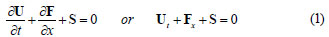
where:
t represents time
x represents longitudinal distance
where:
A is the cross-sectional area of flow
u the velocity, g the gravitation acceleration
Fh the hydrostatic pressure force term
Sf the friction slope, and S0 the bed slope
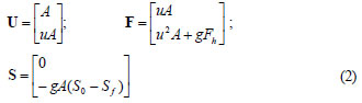
The friction slope is computed by the Manning formula:
where:
nc is the Manning coefficient
R the hydraulic radius.
The hydrostatic pressure force term may be expressed as:

where:
h is the flow depth
η the integration variable indicating distance from channel bottom
W(η) the water-surface width at distance η from the channel bottom
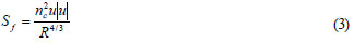
The hydrostatic pressure force term for rectangular and trapezoidal channels becomes:
where:
bw is the base width of channel
z the side slope of the channel.
The governing equations are based on the assumption of hydrostatic-pressure distribution, incompressibility of water, sufficiently small bottom slope of the channel, and negligible wind stress and Coriolis force. Eq. (1) can be expressed in quasi-linear form as:
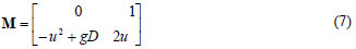
where:
is the Jacobian matrix and D = A/W (η) is the hydraulic depth.
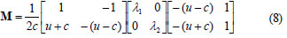
Furthermore, since the matrix M has independent and real eigen-vectors, it can be written in diagonalised form as:
where:
c is the wave celerity expressed as , and the λi values are eigen-values of M giving the characteristic directions.
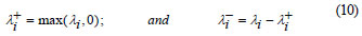
The eigen-values are given by:

The matrix M can now be split into 2 components, positive and negative, by the testing sign of the eigen-values. This may be done as follows:
M = M+ + M-
where:
Beam and Warming scheme
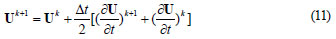
The finite-difference approximation for flow variables U at the higher time level, i.e.: Uk+1, can be written as (Beam and Warming, 1976; Chaudhry, 1993; Jha et al., 1994):
By substituting the value of Ut from Eq. (1) into Eq. (11):
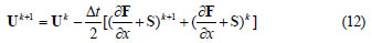
The terms Fk+1 and Sk+1 in Eq. (12) are nonlinear and may be linearised as follows. The Taylor series expansion of Fk+1 may be written as:
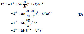
Similarly:

where:
M and B are the Jacobians of F and S with respect to U, respectively.
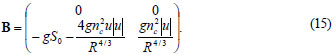
The matrix M in Eq. (7) is replaced in the Eq. (13) and B is given as:
Substituting Eqs. (13) and (14) into Eq. (12) and simplifying
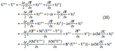
Therefore:
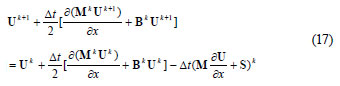
Introducing the split form of matrix M, as given by Eq. (10), Eq. (17) is written as

where:
I = α (2 x 2) unit matrix.
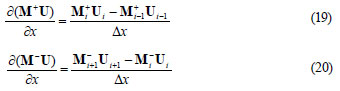
The expressions in the parentheses before Uk+1 and Uk are operators on Uk+1 and Uk respectively, not simple products. The space derivatives associated with positive and negative components of M are approximated by backward and forward space differences, respectively. Therefore:
Multi-grid algorithms
Multi-grid algorithms have become a common approach for solving many types of linear problems of the form Gx = b. In order to describe the multi-grid algorithm, let Ω be the domain of problem (1). To approximate  , we consider a sequence of subintervals Ωj of Ω determined by a regular subdivision; namely, the set Ω is divided into 2j equi-distant subintervals at levelj = 1,2, ..., J. In addition, we denote Gj as the generated matrix by Beam-Warming scheme at the level j and at the finest level j=J we define GJ = G. Moreover, we consider
  as an operator from the coarse grid Ωj-1 to the fine grid Ωj. Furthermore, we define Rj as a smoothing operator for level j . For example, in the Jacobi relaxation scheme, Rj is defined D-1 where Dj is the diagonal matrix of G. We denote an approximation of the exact solution x by v and the error, e = x - v by e. Defining the residual by r = b - Gv, we observe the critical relationship known as the residual equation, namely Ge = r. In brief, there is a recursive application of the 2-grid process. First, an iterative method such as the Jacobi or Richardson relaxation is applied to the fine-grid problem. These iterations have the property that after relaxation the error will be smooth. This in turn means that the error can be accurately represented on a coarse grid. Since the coarse grid is much smaller than the fine grid, it is much less expensive to work on the coarse grid. These facts permit the second part of the process, known as the coarse-grid correction. The fine-grid residual rj at the level j is computed and restricted to the coarse grid rj-1 = rj at the level j-1, where it is used as the righthand side of the coarse-grid residual equation Gj-1ej-1 = rj-1. This equation is solved and the error thus determined is then interpolated back to the fine grid, where it is used to correct the fine-grid approximation, vj ← vj+ Ij-1ej-1. By recursively solving the coarse-grid equation with this 2-grid process, a multi-grid algorithm is defined. Now we are ready to state the multi-grid algorithm (Bramble and Pasciak, 1987; Bramble et al., 1991).
Multi-grid algorithm
MG(j, xº, bj) is the approximate solution of the equation
Gj x = bj
Obtained from the jth level iteration with initial guess xº. At the finest level J, set bj: = b and Gj : = G
For j 0, MG(0, xº, b0) is the solution obtained from a direct method. In other words,
MG(0, xº, b0) = 
We note that b0 is determined recursively by Step (2) in the following error correction step. For j > 1, MG(xº, bj) is obtained recursively in 7 steps.
Pre-smoothing step:
1 Define xl for l = 1,...,m by
xl = x1-l + Rj (bj - Gjx 1-1).
Error correction step:
2. Set bj-1 =  (bj - Gjx m). (Transformation of residual from fine grid j to coarse grid j-1.)
3. Set qº = 0.
4. (Solving the residual equation) For i = 1,...,p defines error corrector
qi = MG (j-1 qi-1, bj-1)
If the residual equation in Step (4) is not solvable directly, set j:=j -1 and go to Step (2). Otherwise:
5. Define xm+1 = xm + qp
6. Define x1 for l = m +1,...,2m by xl+1 = x1 + Rj (bj - Gjx l).
If j ≠ J, set m: = 2m +1 and go to Step (5). Otherwise:
7. Define MG (J, xº, b) = x2m.
In this algorithm, m is a positive integer which may vary from level to level and determines the number of pre- and postsmoothing iterations. If p = 1, we have a V-cycle multi-grid algorithm. If p = 2 , we have a W-cycle algorithm. A variable V-cycle algorithm is one in which the number of smoothing m increases exponentially as j decreases (i.e., p = 1 and m = 2J-j). The above multi-grid is called a symmetric multi-grid algorithm. If the post-smoothing step is removed, it is called a non-symmetric multi-grid algorithm.
Block multi-grid algorithm for Beam-Warmingscheme
The differential equation can aid in forming a prolongation operator (Trottenberg et al., 2001). In this section, we use the Beam-Warming scheme to form the interpolation (prolongation) operator. To this end, let : Ωj-1 → Ωj be a mapping from the coarse grid Ωj-1 to the fine grid Ωj. We also assume that:
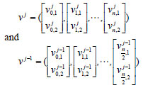
are defined on Ωj and Ωj-1 , respectively. To construct the prolongation operator, the values of coarse-grid points will be transformed unchanged, i.e.:
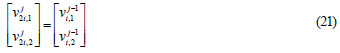
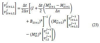
for 0< i < . To construct a non-standard mapping on the middle points, one can use the Beam-Warming scheme. For this purpose, we first denote wk as the value of wat time tk:
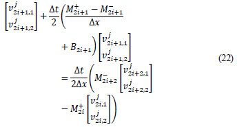
Hence, by Eqs. (21) and (22) we have:
In addition, the restriction operator, = 2 ()T is used.
Remark: It is clear that the number of required arithmetic operations to construct this operator is more expensive than the standard operator. However, this is not so important because, the inter-grid transfer operators are only constructed once. The expense of running some systems by the multi-grid Beam-Warming scheme involving this new inter-grid transfer operator is much lower than for the ones involving standard operators.
Now, we want to give an extension of the above inter-grid transfer operator to a 2- dimensional case. To this end, let us consider (●) as the coarse grid points (see Fig. 1). We note that any vector is defined on the grid points. A prolongation operator from coarse level j - 1 to the fine level j can be given by:
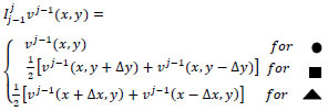
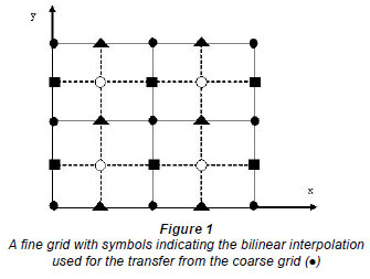
Also, constructing a non-standard mapping on (○) can be done in a way similar to Eq. (23).
Gauss-Seidel block-wise type iteration (relaxation)
In this subsection, we state a smoothing iteration for the Beam- Warming scheme. First, we note that the structure of matrix G in the Beam-Warming scheme (Eq. (18)) is as follows:
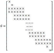
Therefore, the matrix G can be shown
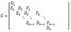
where:
Di, i = 1,2,..., n and Ei, Fi i = 2,3,..., n are 2x2 matrices.
Let us to denote X= [X1, X2,..., Xn]T and b [b1, b2,..., bn]T which X1nd bi are 2 x 1 vectors. Now, in order to apply the smoothing iterations for Beam-Warming scheme, one can use the Gauss-Seidel block-wise iteration for the system Gx = b by:

were
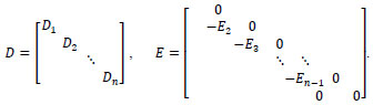
We note that D - E is a lower triangular bi-diagonal matrix and its inverse is easily computable. A simplified form of the above Gauss-Seidel block-wise iteration for the Beam-Warming scheme reads as follows:
Gauss-Seidel block-wise algorithm for Beam- Warming scheme
1. X(º) = 0
2. for l = 2,1,...
3. X1(l)=  b1
b1
4. Xn(l)=  bn
bn
5. for l = 2,3,...,n-1
6. X1(l) = 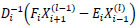
Now, in order to clarify multi-grid algorithm for Beam- Warming scheme, we present the 2-grid algorithm as follows:
Two-grid algorithm for Beam-Warming scheme
(system of G1X=b )
1. Set X(º) = 0
2. Define x1 for l = m 1,...,m by x(l+1) = xl-1 + (D-E) -1 (b - G1x (l-1)).
3. Set r1 = b G1x m).
4. r0 =  . (transformation of the residual from the fine level to the coarse level)
5. Solve G0e0 = r0 directly (i.e. e0 =  ) (solving the system at the coarse level directly)
6. Set e1=  (transformation of the solution in the coarse grid to the fine grid)
7. Set X(m+1) = X(m)+ e1. (modifying of the initial solution in the fine grid)
8. Define X(l) for l = m 1,...,2m by x(l+1) = x(l) + (D-E) -1 (b - G1x (l)).
In the above algorithm, as already mentioned, G0 and G1 denote the system produced by the Beam-Warming scheme in the coarse and fine grids, respectively. We recall that other relaxation schemes such as incomplete LU factorisation can be applied here.
Numerical applications
In order to evaluate the accuracy of the block multi-grid algo rithm for the Beam-Warming scheme, we first solved a classic open-channel shock wave propagation problem. The numerical properties were analysed and illustrated by 2 different examples. Both examples were solved by Matlab 7.5. Since in the high levels (level 3 upwards), matrix G (which it is obtained by the Beam and Warming scheme) cannot be stored in the computer, we stored matrix G by some block matrices whose numbers depend on the level they are in. Therefore, there is no explicit matrix G and there are merely a number of block matrices, the combinations of which would create matrix G.
In both examples, the V-cycle algorithm is used, in which the number of iterations in pre- and post-smoothing processes has been taken as m = 2 for each level j.
Example 1
The hydraulic events following the sudden closure of a gate in a channel are important for designing power channels. For example, the gates of a power channel may be closed instantaneously, which causes an increase in the flow depth. In these situations, the knowledge of the height of the resulting surge is essential for designing a channel.
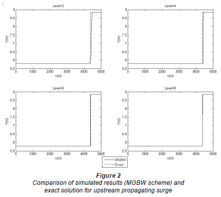
In this example, the performance of the multigrid Beam and Warming (MGBW) scheme for surge propagation due to sudden closure of a gate is examined in comparison with the exact solution. We considered a channel with a rectangular crosssection, the bottom of which is 6.1 m wide. The initial conditions in the channel are: 5.79 m deep with a steady discharge of 126 m3·s-1. The channel is horizontal and frictionless with a length of 5 km. The water surface level in the reservoir is constant at the upstream end and the sluice gate at the downstream end of the channel is suddenly closed at time t = 0.
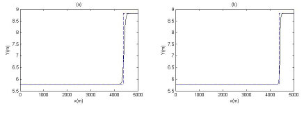
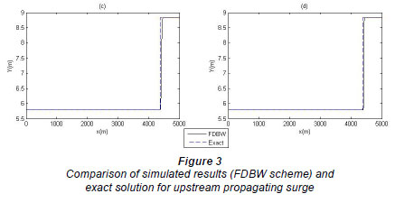
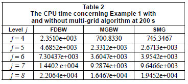
Figure 2 shows the simulated results by the MGBW scheme with the exact solution (Featherstone and Nalluri, 1995) just 90 s after gate closure for different levels. The finest level is considered J=8, and also at the coarsest level, the grid size in space Δx and in time Δt are taken as 25 m and 2.2514 s, respectively. Hence, the system produced by the Beam-Warming scheme at the coarsest level (J=1) has 202 x 202, and at the finest level (J=8) 25 602 x 25 602 dimensions at any time level. It can be seen that the MGBW scheme is in a good agreement with the exact solution. Figure 3 shows the simulated results by the finite-difference Beam and Warming (FDBW) scheme (Chaudhry, 1993) with the exact solution. In this figure, we considered (a) Δx = 25 and Δt = 2.2514, (b) Δx = 12.5 and Δt = 1.1257, (c) Δx = 6.25 and Δt = 0.5629, (d) Δx = 3.125 and Δt = 0.2814. Figures 3a, 3b, 3c and 3d correspond to levels 1, 2, 3 and 4 of MGBW scheme, respectively. In this example, the simulated results are satisfactory and hence this scheme is valid. Let and be the approximated solution obtained by MGBW and exact solution, respectively. Table 1 shows the Euclidean error norm  for different times from level j=3 to j=8. As we can see, when the level increases, the value of error decreases significantly. In addition, we examined this example without the multi-grid scheme. The CPU time concerning the perfor mance in Example 1 by the MGBW and FDBW schemes at 200 s is given in Table 2. The stop criterion for FDBW is
  . In Table 2, MGBW and SMG denote the Beam-Warming and standard inter-grid transfer operators applied to the Gauss-Seidel algorithm, respectively. The standard inter-grid transfer operator that we used is the injection operator. As we observe, the CPU time decreases significantly from level 4 to the end when we use multi grid scheme. Moreover, in the second and third columns we see that the MGBW algorithm is run faster than the SMG algorithm. Table 2 shows the efficiency of the multi-grid algorithm, clearly.
Example 2
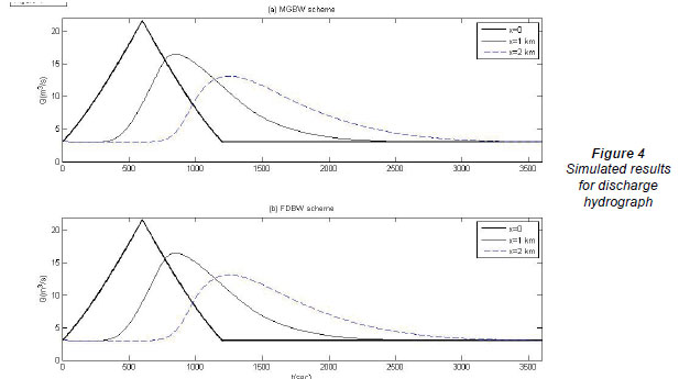
Because flood waves normally have a rising limb, a falling limb and a single peak similar to a triangular hydrograph, the latter is usually used as an input function for flood routing analysis. This example is presented for a case of subcritical flow in a rectangular channel with the length of L = 20 km, width of 6 m, uniform bottom slope of S0 = 0.00193 and a roughness defined by the Manning nc = 0.025 m-1/3 s. Also, uniform flow with a depth of 0.5 m and velocity corresponding to Froude number Fr = 0.5 are considered for the initial conditions. The upstream boundary conditions are defined by a triangular hydrograph Q = Q(t) which changes linearly from 3 to 21.57 m3·s-1 in 600 s and then decreases to 3 m3·s-1, again in 600 s. The downstream boundary conditions are: h = h(t) = const.
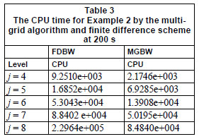
In Fig. 4, Q = Q(t) for the sections x = 1 000 and 2 000 m at the level j=3 with Δx = 10 m and Δt = 3 s, is given by the MGBW and FDBW schemes. Hence, the system resulting from the Beam-Warming scheme at the coarsest level (J=1) has 1002 x 1002, and at the finest level (J=8), 128002 x 128002 dimensions at any time level. The CPU time for Example 2 by the MGBW and FDBW schemes at 200 s is given in Table 3. We considered n=500 iterations for the FDBW scheme in any time. table 3 shows that the MGBW scheme is run faster than the FDBW scheme.
Conclusions
This paper presents a numerical analysis of the MGBW scheme applied to the complete Saint-Venant equations written for 1-dimensional unsteady flow. Solving the Saint-Venant problem by the Beam and Warming scheme concludes a linear system Gx = b. In order to find a good solution, we need to use a very small size for the grid in terms of space (Δx) and time (Δt). Then, the dimension of G would be very large and saving this matrix in a computer is impossible. Hence, most of the iterative methods cannot be used. MGBW has been used to solve the problem. The main factor that influences the convergence rate of the multi-grid continuation algorithms is the distance between the solutions provided by different meshes. MGBW significantly reduces the computational time. The MGBW scheme may be expected to give accurate results for other unsteady open-channel flow problems, such as those involving propagation of a flood wave in a natural stream or flow in a transition.
Acknowledgments
The authors would like to thank the anonymous referees for their valuable comments and suggestions. Also, the second author gratefully acknowledges the financial support by the Vali-e-Asr University of Rafsanjan, Iran (Grant No. p/1453).
References
ABBOTT MB (1979) Computational Hydraulics. Pitman Publishing, London. [ Links ]
AURELI F, MARANZONI A, MIGNOSA P and ZIVERI CA (2008) Weighted surface-depth gradient method for the numerical integration of the 2D shallow water equations with topography. Adv. Water Resour. 31 962-974. [ Links ]
BEAM RM and WARMING RF (1976) An implicit finite-difference algorithm for hyperbolic systems in conservation-law form. J. Comput. Phys. 22 87-110. [ Links ]
BRAMBLE J and PASCIAK J (1987) New convergence estimates for multigrid algorithms. Math. Comput. 49 311-329.
BRAMBLE J, PASCIAK J and XU J (1991) The analysis of multigrid algorithms with non-nested spaces or non-inherited quadratic forms. Math. Comp. 56 1-34. [ Links ]
BRAMBLE JH (1993) Multigrid Methods. Pitman, London. [ Links ] CATELLA1 M, PARIS E and SOLARI L (2008) Conservative scheme for numerical modeling of flow in natural geometry. J. Hydraul. Eng. 134 (6) 736-748. [ Links ]
CHAUDHRY MH (1993) Open-Channel Flow. Prentice-Hall, Englewood Cliffs, NJ. [ Links ] CHOI GW and MOLINAS A (1993) Simultaneous solution algorithm for channel networks modeling. Water Resour. Res. 29 (2) 321-328. [ Links ] CHOW V (1959) Open Channel Hydraulics. McGraw-Hill, Auckland. [ Links ]
FEATHERSTONE RE and NALLURI C (1995) Civil Engineering Hydraulics. Blackwell Science Ltd, Oxford. [ Links ] JHA AK, AKIYAMA J and URA M (1994) Modeling unsteady open channel flows modification to Beam and Warming scheme. J. Hydraul. Eng. 120 (4) 461-476. [ Links ]
NGUYEN QK and KAWANO H (1995) Simultaneous solution for flood routing in channel networks. J. Hydraul. Eng. 121 (10) 744-750. [ Links ]
SEN DJ and GARG NK (2002) Efficient algorithm for gradually varied flows in channel networks. J. Irrig. Drain. Eng. 128 (6) 351- 357. [ Links ]
TAVAKOLI A and KERAYECHIAN A (2007) Improvement of the rate of convergence estimates for multigrid algorithm. App. Math. Comput. 187 922-928. [ Links ]
TAVAKOLI A (2010) Convergence of multigrid algorithms in divergence free space for Stokes problem. Int. J. Appl. Math. Mech. 6 (3) 62-76. [ Links ]
TROTTENBERG U, OOSTERLEE CW and SCHULLER A (2001) Multigrid. Academic Press, New york. [ Links ]
TSENG MH and CHU CR (2000) The simulation of dam-break flows by an improved predictor-corrector TVD scheme. Adv. Water Res. 23 637-643. [ Links ]
VENUTELLI M (2002) Stability and accuracy of weighted four point implicit finite difference schemes for open channel flow. J. Hydraul. Eng. 128 (3) 281-288. [ Links ]
Received 8 March 2010; accepted in revised form 7 March 2011.
* To whomall correspondence should be addressed. +98 913 199 0614; fax: +98 341 3220733; e-mail: rahimpour@mail.uk.ac.ir

