TECHNICAL PAPER

 

A new method for long-term safety analysis of marine structures

 

 

Y G Wang

Correspondence

 

 

---

ABSTRACT

This paper proposes to utilise a new adaptive kernel density estimation (KDE) method based on a linear diffusion process for fitting the significant wave height data in order to calculate the sea state parameter distribution tails more accurately, particularly the higher, more extreme values. The accuracy of the proposed method has been demonstrated based on fittings to two measured ocean wave datasets. This proposed method has subsequently been utilised for deriving accurate 50-year and 500-year environmental contour lines. The advantages of using a more reliable contour line derived from using the proposed new method for long-term safety analysis of marine structures have been substantiated.

Keywords: marine structures, adaptive kernel density estimation, linear diffusion process, long-term, dynamic analysis, sea severity

---

 

 

INTRODUCTION

Describing sea severity statistically provides vital information for the design, installation and operation of marine structures. To successfully design a marine structure, one needs information on the roughest, most extreme sea state that the structure will meet during its design life (e.g. 50 years). In general, the available sea severity information is a data set of significant wave height (H_s) measured at a sea site over a relatively short span of time (e.g. 25 years or less). For predicting the extreme H_s value that the marine structure is expected to encounter at a specific sea site in 50 years or more, depending on the design or operational requirements, it is necessary to first find a suitable probability distribution that represents the measured data accurately. In the existing literature, the three-parameter Weibull model is the most widely used probability distribution for the significant wave height H_s). Based on the information of the fitted marginal distributions of H_s and a specific wave period and their correlation structures, an environmental contour (an environmental contour describes the tail properties of some relevant environmental variables, and is used as input to the design process) line corresponding to a design life cycle time period (e.g. 50 years) can be generated by using a suitable transformation between the normal space and the physical space.

Clarindo et al (2021) explored the use of the Monte Carlo Importance Sampling technique to reduce the variance on the probability of failure estimates based on prior information on the environmental contour provided by the classic IFORM (Inverse First-Order Reliability Method) approach. The IFORM is a widely used approach for calculating environmental contours based on the joint probability distribution of the environmental variables, and the Rosenblatt transformation is a common approach to establish the transformation between the variable space and the standard normal space within which the environmental contour is calculated based on common exceedance probability. In the Clarindo et al (2021) study, the joint environmental model of the sea waves was described by the marginal three-parameter Weibull distribution of significant wave height (H_s) and by the conditional log-normal distribution of the wave period fitted to a large collection of simulated wave data. It was shown that the IFORM approach gives quite smooth environmental contour lines. Haselsteiner et al (2021) presented an approach to reduce the conservatism associated with highest density environmental contours. In their calculation example of an environmental contour for sea states, they assumed that the significant wave height follows a three-parameter Weibull distribution. It was found in their study that when the 50-year response is estimated, the IFORM method can lead to non-conservative response estimates of a marine structure. Mackay and Haselsteiner (2021) studied the relationship between the marginal exceedance probability of the maximum value of each sea state variable along an environmental contour and the total probability outside the contour. To illustrate the relationship between marginal and total exceedance probabilities and quantiles (quantiles are values that split sorted data or a probability distribution into equal parts; in general terms, a q-quantile divides sorted data into q parts) in a realistic case, they used a sea state model in which the significant wave height is assumed to follow a three-parameter Weibull distribution. In their research, they obtained environmental contours by using a suitable transformation between the normal space and the physical space based on the Inverse First-Order Reliability Method (IFORM). In Wrang et al (2021), 50-year environmental contours were generated for four study sites located in the North Sea, Skagerrak and the Baltic Sea by considering both observations and hindcast (model) data. For the construction of the contours, the well-established IFORM approach and a modified version using principal component analysis (PCA) were both examined. In the implementation of the IFORM method in Wrang et al (2021), the marginal probability distribution of the significant wave height was taken as a three-parameter Weibull distribution. It was found that a version of the regular IFORM was able to produce satisfactory contours. When using PCA, the dependency in the data was not properly captured by the probability functions under consideration. The system reliability of a semi-submersible platform was estimated in the study of Zhao and Dong (2022a). In this study environmental contours were calculated using the IFORM method in which the marginal distribution for the significant wave height was fitted using a three-parameter Weibull distribution. Zhao and Dong (2022a) pointed out that, "Those probabilistic expressions obtained from environmental contour-based values can be used for preliminary design evaluation of floating structures, which can be used to address the design loads and failure probability of the entire system" Zhao and Dong (2022b) presented an extension of the alternative environmental contour approach based on inverse first-order reliability theory in a three-dimensional model that accounts for short-term extreme response uncertainties. In their study, for constructing an environmental contour, a marginal distribution for the significant wave height was fitted to a three-parameter Weibull distribution. In their research work they concluded that, "The environmental contour method that uncouples the structural response and environmental variables is efficient, whereas the design loads results can be inaccurate and unconservative compared with those derived from the long-term loads models" Chai and Leira (2018) extended the IFORM approach to estimate inverse second-order (ISORM) environmental contours. However, their ISORM contour method is still based on the Rosenblatt transformation of the parametric marginal model (three-parameter Weibull distribution) of the significant wave height (H_S).

In all the above-mentioned open literature the three-parameter Weibull model is the chosen distribution for the significant wave height when developing environmental contours. However, the problems or limitations in the above-mentioned literature are that these authors have not investigated the performances of the three-parameter Weibull distribution for fitting the probability distribution tails. Haselsteiner and Thoben (2020) noticed that, "In the design process of marine structures like offshore wind turbines, the long-term distribution of significant wave height needs to be modelled to estimate loads. This is typically done by fitting a translated Weibull distribution to wave data" However, being doubtful about the suitability of the translated Weibull distribution (three-parameter Weibull distribution), these authors analysed wave datasets from six locations suitable for offshore wind turbines. Three datasets were derived from moored buoys off the US East Coast and three datasets were gathered from a hindcast that covers the North Sea. In their research, they found that, in all six datasets, the three-parameter Weibull distribution predicts too low probability densities in the tail and consequently also too low quantiles in the tail.

It should be noted that all the afore-mentioned studies applied the parametric method for fitting the probability distribution of the significant wave height. Haselsteiner et al (2017) used a nonparametric kernel density estimation (KDE) method to calculate the probability distributions, and to predict environmental contours of extreme sea states. Kernel density estimation is the process of estimating an unknown probability density function using a kernel function. While a histogram counts the number of data points in some-what arbitrary regions, a kernel density estimate is a function defined as the sum of a kernel function on every data point. However, Ross et al (2020) pointed out that the ordinary kernel density estimation method is not a good choice to describe the probability distribution tails. Eckert-Gallup and Martin (2016) applied the bivariate kernel density estimation with Abramson's adaptive bandwidth selection method in their estimation of environmental contours of extreme sea states. Although the method in Eckert-Gallup and Martin (2016) can well capture the probability distribution tails and accurately predict environmental contour lines, the Abramson's adaptive bandwidth selection in Eckert-Gallup and Martin (2016) is both difficult to implement and computationally expensive. Thus, seeking a more efficient adaptive bandwidth selection process for the KDE method is needed in order to capture the probability distribution tails and predict environmental contours more accurately and more efficiently.

Aiming to overcome the deficiencies of all the aforementioned parametric and nonparametric approaches, this paper proposes to utilise a new adaptive kernel density estimation method based on a linear diffusion process which can help to capture the probability distribution tails more accurately and efficiently. The proposed new adaptive kernel density estimation method will be utilised in calculating the distribution tails of a measured H_S data set at NDBC (National Data Buoy Center) Station 46012 and another measured H_s data set at NDBC 44007 operated by the US National Oceanic and Atmospheric Administration. Through comparing with the prediction results obtained using a parametric method, an ordinary KDE method and the Abramson's adaptive KDE method, the accuracy and efficiency of the proposed new adaptive KDE method will be substantiated. Next, the proposed new adaptive KDE method and the Rosenblatt-ISORM method will respectively be applied for calculating 50-year environmental contour lines based on the above-mentioned measured NDBC 46012 data set. These obtained contour lines will subsequently be used in calculating the 50-year design force values for a typical marine structure (in this case, a point absorber wave energy converter). Through analysing and comparing the calculation results, the advantages of using the proposed new adaptive KDE method for long-term safety analysis of marine structures will be substantiated.

 

THEORETICAL BACKGROUND

Theories behind the traditional IFORM and ISORM contour approaches

For the dynamic analysis of a specific marine structure, the long-term response extremes of the structure can be obtained by resorting to a short-term analysis based on the environmental contour line method (Haver & Winterstein 2009). The environmental contour line method can be applied for an ocean site if the marginal probability distribution of the H_s and the conditional probability distribution function of the wave period are both available.

The first step for deriving an environmental contour line is to apply the following two Rosenblatt transformation equations to transform the marginal and conditional probability distributions to a standard Gaussian space (the u₁ u₂ space):

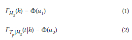
Where:

Fh (h) is the marginal probability distribution of H_s

Ft_p \h (t|h) is the conditional probability distribution of the peak spectral period (T_p)

Φ( ) is the cumulative distribution function of the standard uni-variate Gaussian distribution.

In the standard Gaussian space, the q annual exceedance probability environmental contour line will be circles having radius r = Φ^-1(1 - q/2 920) where 2 920 is the number of the three-hour sea states in each year. The radius r from the origin to the design point, referred to as the reliability index, is also denoted by ß_F in the existing literature. If q/2 920 is denoted as α, the relation Φ(β_F) = 1 - α will be derived. The q-probability environmental contour lines can then be obtained by transforming these circles in the standard Gaussian space back to the original physical space using the following inverse Rosenblatt transformation equations (see e.g. Manuel et al 2018) :

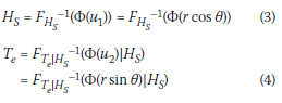
The whole environmental contour line can be derived by varying the angle θ in Equations 3 and 4 from 0 to 2π. The derivation process in Equations 1 to 4 for obtaining an environmental contour line is called the Inverse First Order Reliability Method (IFORM). Mackay and Haselsteiner (2021) pointed out that, for an IFORM environmental contour at exceedance probability α, the maximum values of the standard Gaussian variables have marginal exceedance probability α in standard Gaussian space. However, the same is not true for the maximum values of original random variables along the IFORM contour in the original physical space.

The IFORM approximation is conservative when the failure region is convex, but is not conservative if the failure region is concave. Chai and Leira (2018) proposed a second-order approximation to the failure surface which is always conservative, and their proposal is called the Inverse Second Order Reliability Method (ISORM). In the ISORM method the failure surface is assumed to enclose a circle in the standard Gaussian space, centered at the origin. The radius β_s2 is defined so that the probability that an observation falls outside the circular region is α. Chai and Leira (2018) noted that, since the sum of two independent standard Gaussian variables follows a Chi-squared distribution on two degrees of freedom x²₂, the radius can be written as:

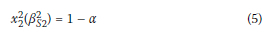
In the ISORM definition, the radius β₅₂ is a function of the exceedance probability. As with the IFORM environmental contour, the ISORM environmental contour in the original physical space is obtained by applying the inverse Rosenblatt transformation to the contour in standard Gaussian space.

The ordinary and Abramson's adaptive kernel density estimation (KDE) methods

The IFORM and ISORM approaches for environmental contours are both parametric methods that require some specific predefined probability distribution models for the sea state parameters. However, a drawback to parametric modelling is that the requirements on the predefined probability model may be too restrictive and rigid for adequately estimating the true underlying function. To overcome the rigidity of the parametric sea state parameter probability distribution models, the non-parametric KDE method can be utilised. The KDE is a fundamental data-smoothing problem solver in which inferences about the population are made based on a data sample of finite size. Suppose (X1, ... X_n) are finite data samples drawn from an unknown univariate probability density distribution f at any given point x. It is of interest to estimate the shape of this function f. Its ordinary kernel density estimator is (Eckert-Gallup & Martin 2016; Silverman 1986):

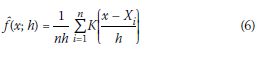
where K is the kernel, a non-negative function satisfying fK(x)dx = 1, and h > 0 is a smoothing parameter called the band-width. A range of kernel functions are commonly used: uniform, triangular, biweight, triweight, Epanechnikov, normal, and others. The Epanechnikov kernel is optimal in a mean square error sense, and therefore it is utilised in this study.

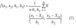
The afore-mentioned univariate kernel density estimator can be extended to the bivariate setting by using two bandwidths (h₁ and h₂), one in each coordinate's direction. Let ... X_n1 be a data sample in one coordinate's direction and X₁₂, ... X_n2 be a data sample in another coordinate's direction. Then the bivariate kernel density estimation can be implemented using Equation 7:

Up to this point the theoretical background for the ordinary kernel density estimation (KDE) with an optimal kernel function has been presented. The ordinary kernel density estimation method can generally provide satisfactory estimates in the central parts of a probability distribution. However, the ordinary KDE usually cannot provide satisfactory estimates of the probability distribution tails, and consequently also does not extrapolate well.

In order to calculate the sea state parameter distribution tails more accurately, and to derive accurate environmental contour lines, Eckert-Gallup and Martin (2016) proposed to use Abramson's adaptive kernel density estimation (KDE) method in which the bandwidth of the kernels is allowed to vary from one point to another. To implement Abramson's adaptive KDE method, a pilot estimate f(x₁ x₂) satisfying fX_li, X_2i) > 0 for all i is first found. One can then calculate the local bandwidth parameters λ_i as follows (Silverman 1986; Wand & Jones 1995):

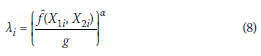
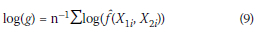
where a is the sensitivity parameter that satisfies 0 < α < 1. In Equation 8, g is obtained using Equation 9:

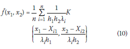
One can then calculate the adaptive kernel estimate f(x₁, x₂) as follows (Silverman 1986):

However, Abramson's adaptive KDE method is both difficult to implement and computationally very expensive. In the next subsection this paper will propose a new adaptive KDE method that can be utilised to capture the sea state parameter probability distribution tails more accurately and efficiently.

Adaptive KDE method based on linear diffusion processes

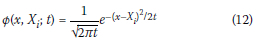
Suppose again that X₁, ... X_n are finite data samples drawn from an unknown univariate probability density distribution f at any given point x. One can derive the Gaussian kernel density estimator as follows (Botev et al 2010):

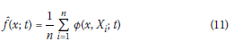
in which

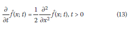
It can be seen that in this case the band-width parameter is Vt. One can see that the Gaussian kernel density estimator (12) can be uniquely obtained by evolving the solution of the following diffusion equation up to time t (Botev et al 2010):

Equation 13 possesses the following initial condition:

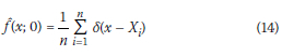
in which δ(χ - Xi) is the Dirac Delta function at X_i. One can extend the diffusion model (13) based on the smoothing properties of the linear diffusion equation (Botevet al 2010):

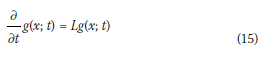
in which L is the linear differential operator that possesses the form 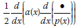and a(x) and p(x) can be chosen to be any arbitrary positive functions that have bounded second derivatives. Equation 15 possesses the following initial condition:

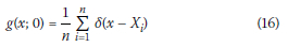
in which δ(χ - X_i) is the Dirac Delta function at X_i. Solving Equation 15 one can obtain (Botev et al 2010):

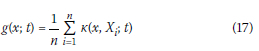
in which the asymptotic approximation κ(χ, X_i; t) is expressed as follows:

The bandwidth parameter Vt is asymptotically optimal and its square is expressed as follows (Botev et al 2010):

in which E denotes mathematical expectation. ||·•| is the Euclidean norm. It can be seen that the t value changes with the value of x. This is why this proposed method is called a new adaptive kernel density estimation method based on linear diffusion processes.

In this subsection a new kernel density estimator based on a linear diffusion process has been presented. It can be seen that the key idea is to construct an adaptive kernel by considering the most general linear diffusion with its stationary density equal to a pilot density estimate. That is to say, the key idea is to view the kernel from which the estimator is constructed as the transition density of a diffusion process. When implementing this method, one utilises the most general linear diffusion process that has a given limiting and stationary probability density. This stationary density is selected to be a pilot density estimate. The approach leads to a simple and intuitive kernel estimator with substantially reduced asymptotic bias and mean square error. The proposed estimator deals well with boundary bias and, unlike other proposals, is always a bona fide probability density function. It can be shown that the proposed approach brings some well-known bias-reduction methods together under a single framework, such as the Abramson estimator. The resulting diffusion estimator unifies many of the existing ideas about adaptive smoothing. In addition, the estimator is consistent at boundaries.

 

A CALCULATION EXAMPLE AND DISCUSSIONS FOR THE H_S PROBABILITY DISTRIBUTIONS

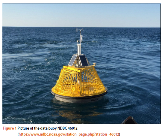
This section provides a calculation example and discussions of the calculation results based on the measured wave data at the National Data Buoy Centre (NDBC) Station 46012 (see the picture in Figure 1). This data buoy is located at Half Moon Bay - 24 nautical miles south-southwest of San Francisco on the United States west coast. This data set contains 180 554 hourly measurements of H_s and energy periods (T_e) taken from 1 January 1996 to 31 December 2021 at the NDBC 46012.

 

 

The water depth at this measured site is 208.8 m, which can obviously be considered as a deep-water depth. According to the classic naval architecture theory, ocean waves at this site will be less affected by the sea bottom and are therefore linear waves.

The calculation results based on the 180 554 hourly measurements of H_s at NDBC Station 46012 are summarised in Figure 2. The red curve in Figure 2 is the fitted three-parameter Weibull distribution using Equation 20:

 

 

 

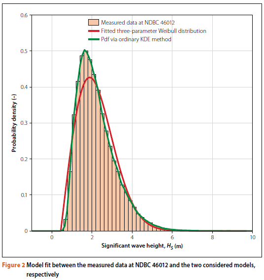
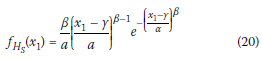
In this case the scale parameter α = 2.0228, the shape parameter β = 2.0167 and the location parameter γ = 0.4422. It can be seen that this red curve fits poorly with the measured data at the mode of the probability distribution. Furthermore, a zoom-in plot in Figure 3 also clearly shows that the red curve fits poorly with and significantly underestimates the measured data at NDBC Station 46012, indicating that the parametric model (the three-parameter Weibull model) is not a good choice to represent the H_s probability distribution.

 

 

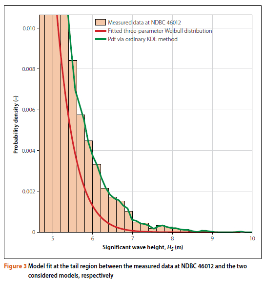
The green distribution curve in Figure 2 has been constructed by using the ordinary KDE method based on the same set of measured H_s data. It can be seen that this green distribution curve fits quite well with the measured data at the mode of the probability distribution. However, the zoom-in plot in Figure 3 shows that this green distribution curve has become zigzagged and fits poorly with the measured H_s data, indicating that the ordinary KDE method is also not a good choice to calculate the H_s probability distribution.

Taking note of the fact that the ordinary kernel density estimation method cannot provide satisfactory prediction results, Abramson's adaptive KDE method was resorted to in order to get better prediction results of the distribution tails. The calculation results using Abramson's adaptive KDE method are represented by the green curves in Figures 4 and 5. It can be seen that the green distribution curve in Figure 4 fits very well with the measured H_s data at the mode of the distribution. In addition, the green distribution curve in Figure 5 also fits very well and fits smoothly with the measured H_s data at the right tail region of the distribution.

 

 

 

 

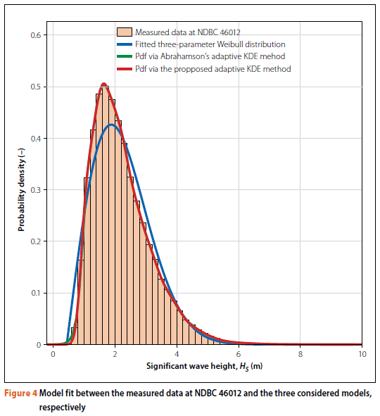
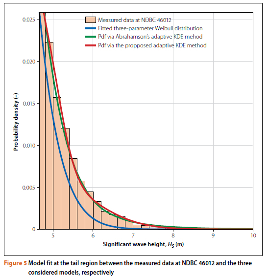
Unfortunately, obtaining the green curve in Figure 4 costs more than 1 827 seconds to run the MATLAB code on a Dell Precision 5820 workstation. This is computationally too expensive, especially for some time-constrained practical engineering projects. Aiming to overcome this deficiency of Abramson's adaptive KDE method, the proposed new adaptive KDE method based on linear diffusion processes was utilised to predict the H_s probability density distribution based on the same set of measured data, and the prediction results are represented by the red curve in Figure 4. It can be seen that this red distribution curve in Figure 4 fits very well with the measured H_s data at the mode of the distribution. In addition, the red distribution curve in Figure 5, obtained using the proposed new adaptive KDE method, also fits very well and fits smoothly with the measured H_s data at the right tail region of the distribution. Furthermore, this red distribution curve in Figure 5 also fits the measured H_s data slightly better than the green distribution curve from using Abramson's adaptive kernel density estimation method. Most impressively, obtaining the red curve in Figure 4 cost only about 34 seconds for running the MATLAB code on a Dell Precision 5820 workstation. This is about 54 times faster than Abramson's adaptive KDE method, indicating that our proposed new method can be utilised to capture the sea state parameter probability distribution tails more efficiently and accurately.

This paper has so far graphically proved the accuracy and effectiveness of our proposed new adaptive KDE method based on linear diffusion processes. Despite the clarity about the accuracy and efficiency of this new method, graphically, this paper now continues to prove the accuracy of this new method by using goodness-of-fit tests such as the Crámer-von-Mises statistic. The Crámer-von-Mises statistic could be used to assess and compare the fits. In statistics the Crámer-von-Mises is a criterion used for judging the goodness-of-fit of a cumulative distribution function F* compared to a given empirical distribution function F. It is defined as:

Let x₁, X₂ ... x_n be the observed values, in increasing order. Then, the Crámer-von-Mises test statistic is:

If the Crámer-von-Mises test statistic value is larger, then the fit of the cumulative distribution function F* to the given empirical distribution function, F_n is poorer. A MATLAB code has been written to calculate the Crámer-von-Mises test statistic value. Based on the measured data (the H_s data in Figures 4 and 5), the Crámer-von-Mises test statistic value for the proposed adaptive KDE estimated distribution (the red curve in Figure 4) was calculated to be 0.0957. Similarly, the Crámer-von-Mises test statistic value for the fitted three-parameter Weibull distribution in Figure 4 was calculated to be 254.4443. Therefore, it has been quantitatively verified that in Figures 4 and 5 the proposed adaptive KDE estimation fits the data better than the three-parameter Weibull distribution.

 

ANOTHER CALCULATION EXAMPLE AND DISCUSSIONS FOR THE H_S PROBABILITY DISTRIBUTIONS

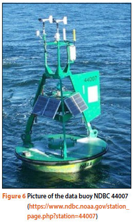
Up until now the new approach proposed in this paper has been applied to one dataset only. In the following section, more information will be provided on the sensitivity analysis conducted on the proposed new method, and how the proposed method performs under different conditions, such as variations in the number of data points. This section will specifically provide another calculation example and discussions of the calculation results based on the measured wave data at NDBC Station 44007 (see photo in Figure 6). This data buoy is located at Portland -12 nautical miles southeast of Portland on the United States east coast. This dataset contains 82 805 hourly measurements of H_s and energy periods (T*_e) taken from 1 January 1996 to 31 December 2005 at NDBC 44007. The water depth at this measured site is 49 m, which is considered to be a shallow water depth. According to classic naval architecture theory, the ocean waves at this site will be more affected by the sea bottom and are therefore nonlinear waves. It is obvious that this measuring site has significantly less data points (82 805) than the measuring site in the first calculation example (180 554). The purpose of this calculation example is to provide more information on the sensitivity analysis conducted on the proposed method. Specifically, the purpose of this calculation example is to discuss how the proposed new method performs under different conditions (i.e. variations in the number of data points).

 

 

The calculation results of the probability densities using Abramson's adaptive KDE method are represented by the green curves in Figures 7 and 8. It can be seen that the green distribution curve in Figure 7 fits better with the measured H_s data at the mode of the distribution than the three-parameter Weibull distribution does. In addition, the green distribution curve in Figure 8 also fits better with the measured H_s data at the right tail region of the distribution than the three-parameter Weibull distribution does. Unfortunately, getting the green curve in Figure 7 costs more than 1 832 seconds for running the MATLAB code on a Dell Precision 5820 workstation. Computationally this is too expensive, especially for some time-constrained practical engineering projects.

 

 

 

 

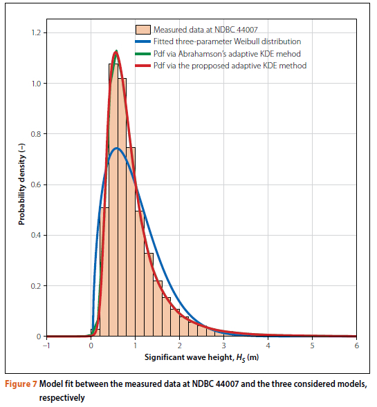
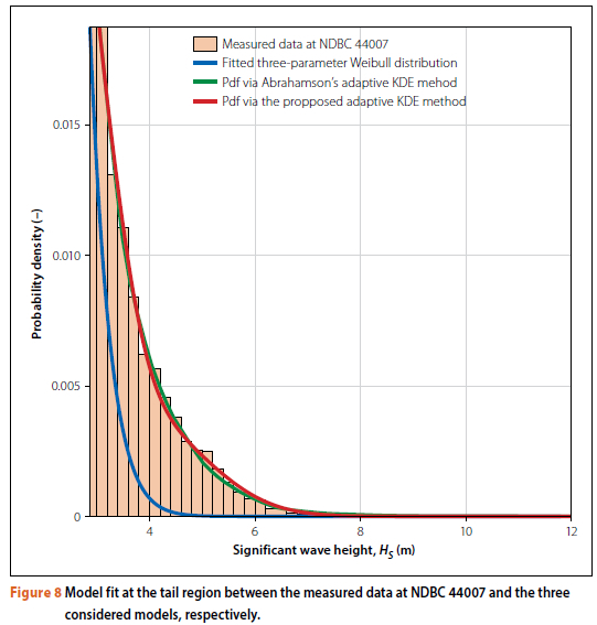
Aiming to overcome this deficiency of Abramson's adaptive KDE method, the proposed new adaptive KDE method, based on linear diffusion processes, was utilised to predict the H_s probability density distribution based on the same set of measured data, and the prediction results are represented by the red curve in Figure 7. It can be seen that this red distribution curve in Figure 7 fits very well with the measured H_s data at the mode of the distribution. In addition, the red distribution curve in Figure 8, obtained using our proposed new adaptive KDE method, also fits very well and fits smoothly with the measured H_s data at the right tail region of the distribution. Furthermore, the red distribution curve in Figure 8 also fits the measured H_s data slightly better than the green distribution curve from using Abramson's adaptive kernel density estimation method. Most impressively, getting the red curve in Figure 7 cost us only about 33 seconds for running the MATLAB code on a Dell Precision 5820 workstation. This is about 56 times faster than Abramson's adaptive KDE method, indicating that our proposed new method can be utilised to capture the sea state parameter probability distribution tails more efficiently and accurately.

In the aforementioned two case studies, two measured datasets with distinct physical properties were used. One dataset was measured at a deep-water site on the United States west coast where the measured waves are linear. Another dataset was measured at a shallow-water site on

the United States east coast where the measured waves are nonlinear. In both case studies the advantages of the proposed new method over the existing methods (the three-parameter Weibull distribution, the ordinary KDE method and the Abramson's adaptive KDE method) have been clearly substantiated. Consequently, the proposed new method is better suited to handle complex data distribution, which is a common challenge in the field.

 

CALCULATION EXAMPLES FOR THE ENVIRONMENTAL CONTOUR LINES

This section first presents the computational results for the 50-year environmental contour lines based on the measured ocean wave data at NDBC 46012.

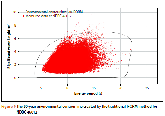
The red "dots" in Figure 9 are the 180 554 hourly measurements of H_s and energy periods (T_e) taken from 1 January 1996 to 31 December 2021 at NDBC 46012. The black curve in Figure 9 is the 50-year environment contour line derived using the IFORM approach. To implement the IFORM approach, the measured H_S data was fitted with a three-parameter Weibull distribution, and the measured T_e data was fitted with a conditional lognormal distribution. After the marginal distribution of H_S and the conditional distribution of T_e were obtained, Equations 1 to 4 were utilised to obtain the 50-year black environmental contour line in Figure 9. One would expect that, for a recording period of 26 years, an environmental contour line with a 50-year return period should include most of the measured data. However, contrary to people's expectations, the black environmental contour in Figure 9 is clearly exceeded by many measured data points that have large H_S values. Consequently, the information provided by the black IFORM contour in Figure 9 will certainly lead to the design of an unsafe marine structure.

 

 

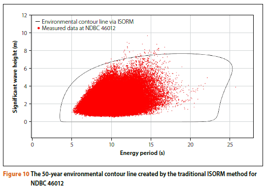
The red "dots" in Figure 10 once again represent the 180 554 hourly measurements of H_S and energy periods (T_e) taken from 1 January 1996 to 31 December 2021 at NDBC 46012. In Figure 10 the black curve represents the 50-year environment contour line forecasted by applying the more conservative ISORM approach. It can be seen that the fitting between the ISORM contour and the measured data set has been slightly improved. Compared to the IFORM contour, the ISORM environmental contour line has missed less of the measured data. However, the ISORM contour still missed a considerable amount of data points that have large H_s values. Consequently, the information provided by the black ISORM in Figure 10 will also lead to the design of an unsafe marine structure.

 

 

As the calculation results from using the IFORM and ISORM methods, based on fitted parametric sea state parameter distributions, were not satisfactory, the proposed new adaptive kernel density estimation (KDE) method was used to derive the environmental contour line. The computational results are presented in Figure 11.

 

 

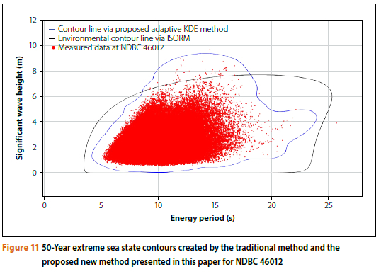
In Figure 11 the blue curve is the 50-year environmental contour line obtained by utilising the proposed adaptive KDE method. Because it has already been shown in Figures 4 and 5 that the proposed adaptive KDE method can well capture the H_s (or T_e) probability distribution tail, and because the blue curve in Figure 11 was directly obtained from the H_s and T_e probability distributions, the blue environmental contour line is certainly more accurate than the black ISORM environmental contour line directly obtained based on the parametric marginal H_s and conditional T_e models that have inaccurate distribution tails. Clearly, this blue environmental contour line should be superior to the black environmental contour line in Figure 11 when being used to predict the extreme values of the dynamic responses of marine structures.

Thus far the proposed new approach in this paper has been applied to derive only the 50-year extreme sea state contour based on the measured dataset at NDBC 46012. In the next section, sensitivity analysis conducted on the proposed new method will also be provided by applying the method to calculate the 50-year, 100-year and 500-year environmental contour lines based on another measured dataset at NDBC 44007.

The red "dots" in Figure 12 are the 82 805 hourly measurements of H_s and energy periods (T_e) taken from 1 January 1996 to 31 December 2005 at NDBC 44007.

 

 

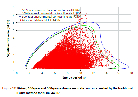
The black curve in Figure 12 is the 50-year environmental contour line derived using the IFORM approach. The green and blue curves in Figure 12 are respectively the 100-year and 500-year environmental contour lines derived using the IFORM approach. One would expect that, for a period of 10 years, an environmental contour line with a 500-year (or 100-year, or 50-year) return period should include most of the measured data. However, contrary to such expectations, the blue (or green, or black) environmental contour line in Figure 12 is clearly exceeded by many measured data points that have large H_s values. Consequently, the information provided by the blue (or green, or black) IFORM contour line in Figure 12 will certainly lead to the design of an unsafe marine structure.

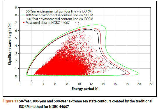
The red "dots" in Figure 13 are the 82 805 hourly measurements of H_s and energy periods (T_e) taken from 1 January 1996 to 31 December 2005 at NDBC 44007. The black curve in Figure 13 is the 50-year environmental contour line derived using the ISORM approach. The red and green curves in Figure 13 are respectively the 100-year and 500-year environmental contour lines derived using the ISORM approach. One would expect that for a period of 10 years, an environmental contour line with a 500-year (or 100-year, or 50-year) return period should include most of the measured data. However, contrary to such expectations, the green (or red, or black) environmentalal contour line in Figure 13 is clearly exceeded by many measured data points that have large H_s values. Consequently, the information provided by the green (or red, or black) ISORM contour line in Figure 13 will certainly lead to the design of an unsafe marine structure.

 

 

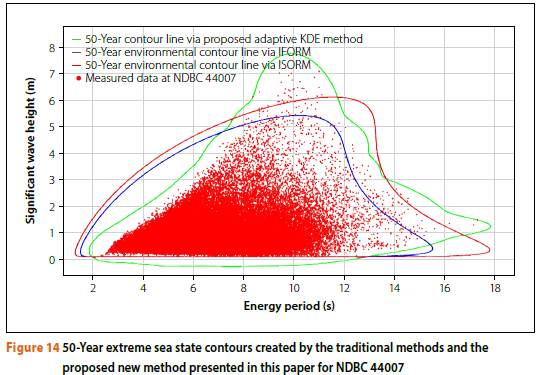
In Figure 14 the green curve is the 50-year environmental contour line obtained by utilising the proposed adaptive KDE method. Because it has already been shown (in Figures 7 and 8) that the proposed adaptive KDE method can well capture the H_s (or T_e) probability distribution tail, and because the green curve in Figure 14 was obtained directly from the H_s and T_e probability distributions, the 50-year green environmental contour line is certainly more accurate than the 50-year red ISORM environmental contour line (or the 50-year blue IFORM environmental contour line) directly obtained based on the parametric marginal H_s and conditional T_e models that have inaccurate distribution tails. Clearly, this 50-year green environmental contour line should be superior to the 50-year red environmental contour line (or the 50-year blue environmental contour line) in Figure 14 when being applied for predicting the extreme values of the dynamic responses of marine structures.

 

 

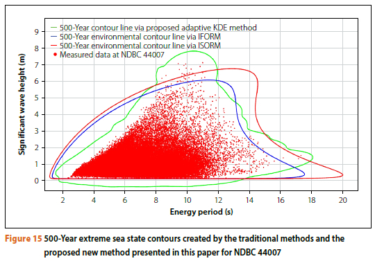
In Figure 15 the green curve is the 500-year environmental contour line obtained by utilising the proposed adaptive KDE method. Because it has already been shown that the proposed adaptive KDE method can well capture the H_S (or T_e) probability distribution tail, and because the green curve in Figure 15 was obtained directly from the H_S and T_e probability distributions, the 500-year green environmental contour line is certainly more accurate than the 500-year red ISORM environmental contour line (or the 500-year blue IFORM environmental contour line) directly obtained based on the parametric marginal H_S and conditional T_e models that have inaccurate distribution tails. Clearly, this 500-year green environmental contour line should be superior to the 500-year red environmental contour line (or the 500-year blue environmental contour line) in Figure 15 when being used to predict the extreme values of the dynamic responses of marine structures.

 

 

A CALCULATION EXAMPLE FOR THE EXTREME RESPONSE VALUES OF A SPECIFIC MARINE STRUCTURE

The chosen marine structure

A specific marine structure - a two-body point absorber wave energy converter (WEC) - was selected for this study. The WEC simulation model, built using the open-source code WEC-Sim (http://wec-sim.github.io/WEC-Sim/), is presented in Figure 16.

 

 

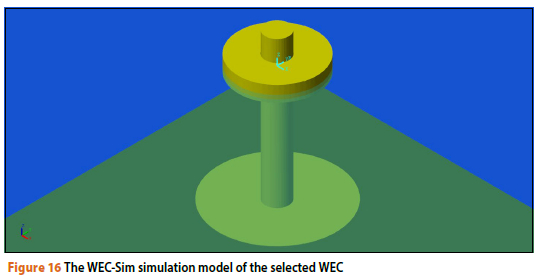
This specific marine structure contains two parts - a spar and a float. The diameters of the spar and the float are 6 metres and 20 metres, respectively. The spar is 38 metres high, and the spar/plate has a mass of 878.3 ton. The float is 5 metres thick and has a mass of 727.01 ton. The draft of this specific marine structure is 82 metres. The marine structure is moored to the seabed using a mooring system consisting of three nylon mooring lines and three anchors. The angle between each pair of mooring lines is 120 degrees in the plan view.

WEC-Sim simulations were conducted to obtain the 50-year extreme PTO (power-take-off) heaving force values of this two-body point absorber WEC in some selected sea states characterised by a Pierson-Moskowitz spectrum (the Pierson-Moskowitz spectral formulation was developed in 1964 from analysis of measured data obtained by Tucker wave recorders installed on weather ships in fully developed seas). Six energy period (T_e) values were selected to define the afore-mentioned sea states along each of the two environmental contour lines in Figure 17, namely 11.06 s, 12.13 s, 14.02 s, 16.43 s, 18.94 s and 23.87 s. These T_e values were selected in order to span the peak H_S values as shown in Figure 17. The black solid "squares" in Figure 17 represent these selected sea states, and their corresponding values are presented in Table 1.

 

 

 

 

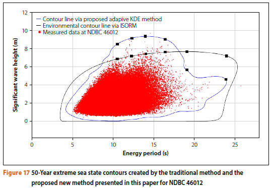
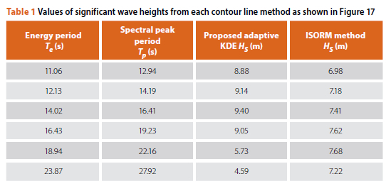
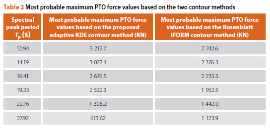
Table 1 shows that the significant wave height estimates using the proposed adaptive KDE method are significantly higher than those derived from the ISORM method. It is therefore obvious that the forces and dynamic responses predicted by the former wave conditions would be larger than those of the latter. In the following, the procedures for deriving the quantitative results of the WEC dynamic responses will be presented. The aforementioned selected sea states, characterised with different PM spectra, were utilised as inputs in the WEC-Sim simulations to obtain the WEC dynamic responses. Specifically, one type of dynamic response, the three-hour time series of the PTO heaving forces that are critical for the WEC design, have been obtained. A most probable maximum PTO force value was subsequently calculated from each three-hour time series of the PTO heaving forces, according to the theory in Edwards and Coe (2019). This procedure was repeated for all the aforementioned six T_e values along each of the two environmental contour lines in Figure 17 to obtain all the most probable maximum PTO force values based on the two environmental contour methods. The calculation results are presented in Table 2. From the prediction results in Table 2 it can be seen that the predicted 50-year extreme PTO force value based on the proposed new adaptive kernel density estimation (KDE) method is 3 212.7 KN, which is much larger than the 50-year extreme PTO force value 2 742.6 KN predicted using the ISORM environmental contour line method. Clearly, the larger 50-year extreme PTO force value predicted utilising the proposed new method will lead to the design of a safer WEC including its PTO device.

 

 

In the following section a more detailed discussion of the practical implications of the proposed new method will be provided. What will be discussed specifically is how the more accurate 50-year environmental contour line derived using the proposed new method can be used to improve the design and safety of a general type of marine structure, and what benefits this may bring in terms of cost savings and risk reduction. Accurate force calculation (by utilising the proposed new method) is of utmost importance in ensuring the structural integrity and safety of a marine structure. The forces acting on a marine structure, such as wave loads, can be incredibly powerful and have the potential to cause significant damage if not properly accounted for. By accurately calculating the forces (by utilising the proposed new method) acting on a marine structure, engineers and designers can ensure that

the marine structure is capable of with-standing these forces and maintaining its stability and functionality, thus reducing maintenance costs. This is especially crucial in marine environments where structures are exposed to harsh environmental conditions. Additionally, accurate force calculation (by utilising the proposed new method) plays a vital role in ensuring the safety of occupants, as it helps to identify potential weaknesses or vulnerabilities in the marine structure that could lead to failures or collapses.

Furthermore, accurate force calculation (by utilising the proposed new method) allows engineers to optimise the use of materials and reduce construction costs. By understanding the exact forces at play, engineers can determine the most efficient design and select appropriate materials to withstand those forces. This not only saves money but also contributes to the sustainability of the marine structure by minimising waste and reducing the environmental impact of construction. Ultimately, accurate force calculation (by utilising the proposed new method) is indispensable in ocean engineering, as it guarantees the durability, safety and cost-effectiveness of the designed marine structure. In conclusion, the proposed new adaptive kernel density estimation (KDE) method can be utilised to predict the design force values for marine structures more efficiently and accurately, and to analyse the design safety of such marine structures.

 

CONCLUSIONS AND FUTURE RESEARCH

In this study, a proposed approach of utilising a new adaptive kernel density estimation (KDE) method based on linear diffusion processes was applied to accurately predict the H_S probability distribution tails of two measured ocean wave datasets. The proposed approach was then applied to derive accurate 50-year and 500-year environmental contour lines that can be utilised in the prediction of long-term design force values for a specific marine structure. In conclusion, the proposed new adaptive KDE method, based on linear diffusion processes, is recommended to predict the long-term extreme dynamic response values for the safe and successful design of marine structures.

In this paper the assumption made in the proposed new adaptive KDE method is that it is based on linear diffusion processes. Numerical experiments have suggested good practical performance by applying this method.

For future research the proposed estimator can be extended in a number of ways. Firstly, one could construct kernel density estimators based on Lévy processes, which will have the diffusion estimator as a special case. Kernels constructed via a Lévy process could be tailored for data for which smoothing with the Gaussian kernel density estimator or diffusion estimator is not optimal. Such cases arise when the data is a sample from a heavy-tailed distribution. Secondly, more subtle and interesting smoothing models could be constructed by considering nonlinear parabolic partial differential equations. One such candidate is the quasilinear parabolic partial differentia equation with diffusivity that depends on the density exponentially. Another viable model is the semi-linear parabolic partial differential equation, and thus the model could be useful for smoothing heavy-tailed data. All such nonlinear models will provide adaptive smoothing without the need for a pilot run, but at the cost of increased model complexity.

 

ACKNOWLEDGEMENT

This work is supported by the National Natural Science Foundation of China (Grant No 51979165).

 

CONFLICT OF INTEREST

There are no conflicts of interest.

 

REFERENCES

Botev, Z I, Grotowski, J F, Kroese, D P 2010. Kernel density estimation via diffusion. Annals of Statistics, 38(5): 2916-2957.         [ Links ]

Chai, W & Leira, B J 2018. Environmental contours based on inverse SORM. Marine Structures: Design, Construction and Safety, 60: 34-51.         [ Links ]

Clarindo, G, Teixeira, A P & Guedes Soares, C 2021 Environmental wave contours by inverse FORM and Monte Carlo Simulation with variance reduction techniques. Ocean Engineering, 228: 1089.         [ Links ]

Eckert-Gallup, A & Martin, N 2016. Kernel density estimation (KDE) with adaptive bandwidth selection for environmental contours of extreme sea states. Proceedings, OCEANS 2016, MTS/IEEE Conference, Monterey, CA.         [ Links ]

Edwards, S J & Coe, R G 2019. The effect of environmental contour selection on expected wave energy converter response. Journal of Offshore Mechanics and Arctic Engineering, 141(1): 011901.         [ Links ]

Haselsteiner, A F, Ohlendorf, J H & Thoben, K D 2017. Environmental contours based on kernel density estimation. Proceedings, 13th German Wind Energy Conference (DEWEK 2017), Bremen, Germany, pp 17-18.         [ Links ]

Haselsteiner, A F& Thoben, K D 2020. Predicting wave heights for marine design by prioritizing extreme events in a global model. Renewable Energy, 156: 1146-1157.         [ Links ]

Haselsteiner, A F, Mackay, E & Thoben, K D 2021. Reducing conservatism in highest density environmental contours. Applied Ocean Research, 117: 102936.         [ Links ]

Haver, S, Winterstein, S 2009. Environmental contour lines: A method for estimating long-term extremes by a short-term analysis. Transactions of the Society of Naval Architects and Marine Engineers, 116: 116-127.         [ Links ]

Mackay, E & Haselsteiner, A F 2021. Marginal and total exceedance probabilities of environmental contours. Marine Structures: Design, Construction and Safety, 75: 102863.         [ Links ]

Manuel, L, Nguyen, P T T, Canning, J & Coe, R G 2018. Alternative approaches to develop environmental contours from metocean data. Journal of Ocean Engineering and Marine Energy, 4: 293-310.         [ Links ]

Ross, E, Astrup, O C, Bitner-Gregersen, E, Bunn, N, Feld, G, Gouldby, B et al 2020. On environmental contours for marine and coastal design. Ocean Engineering, 195: 106194.         [ Links ]

Silverman, B W 1986. Density Estimation for Statistics and Data Analysis. Monographs on Statistics and Applied Probability. London: Chapman and Hall.         [ Links ]

Wand, M P & Jones, M C 1995. Kernel Smoothing. London: Chapman and Hall.         [ Links ]

Wrang, L, Katsidoniotaki, E, Nilsson, E, Nilsson, E & Rutgersson, A 2021. Comparative analysis of environmental contour approaches to estimating extreme waves for offshore installations for the Baltic Sea and the North Sea. Journal of Marine Science and Engineering, 9(1): 1-24.         [ Links ]

Zhao, Y L & Dong, S 2022a. Design load estimation with IFORM-based models considering long-term extreme response for mooring systems. Ships and Offshore Structures, 17(3): 541-554.         [ Links ]

Zhao, Y L & Dong, S 2022b. Comparison of environmental contour and response-based approaches for system reliability analysis of floating structures. Structural Safety, 94: 102150.         [ Links ]

 

 

Correspondence:
Y G Wang
School of Naval Architecture, Ocean and Civil Engineering, Shanghai Jiao Tong University
800 Dong Chuan Road, Minhang District, Shanghai, China 200240
E: wyg110@sjtu.edu.cn

 

 

 

DR YINGGUANG WANG is currently an Associate Professor in the School of Naval Architecture, Ocean and Civil Engineering at Shanghai Jiao Tong University, China. From August 2000 to December 2001 he worked as a graduate research assistant at the University of Washington in Seattle, United States of America. He is both a member of the American Society of Mechanical Engineers and a member of the American Society of Civil Engineers. He is also the Associate Editor of the SNAME Journal of Ship Production and Design. In 2018 he received the prestigious Albert Nelson Marquis Lifetime Achievement Award.