STATISTICS @ WJCM

 

Making sense of regression models in clinical research: a guide to interpreting beta coefficients and odds ratios

 

 

Okechinyere Achilonu; Nneamaka O. Echendu; Glory Chidumwa

Division of Epidemiology and Biostatistics, School of Public Health, Faculty of Health Sciences, University of the Witwatersrand

Correspondence

 

 

---

ABSTRACT

Regression models play a central role in clinical research by quantifying the relationship between outcomes and explanatory variables. Accurate interpretation of model outputs, such as beta coefficients in linear regression and odds ratios in logistic regression, is critical for drawing valid conclusions. This article focuses on the key principles for interpreting linear and logistic regression results in clinical research. A publicly available heart disease dataset was used to demonstrate this. Linear regression was applied to a continuous outcome (cholesterol), while logistic regression modelled a binary outcome (presence of heart disease). Model building involved purposeful variable selection to account for confounding. Model adequacy and multicollinearity were assessed using goodness-of-fit statistics and variance inflation factors, respectively. Interpretation of results focused on beta coefficients and odds ratios. Regression models are robust methods for analysing clinical data and identifying key predictors. The concepts presented in this manuscript provide a foundational framework for applying and understanding linear and logistic regression in clinical research.

---

 

 

INTRODUCTION

Regression models play a fundamental role in clinical research, providing a statistical framework to understand the relationships between a clinical outcome of interest (response or dependent variable) and one or more explanatory variables (also called predictors, exposure, or risk factors) that the researchers choose to evaluate.(1-4) For instance, whether estimating how age affects blood pressure or determining which patient characteristics predict clinical complication status, regression analysis helps researchers derive meaningful and quantifiable insights from data.

Understanding the nature of the outcome variable is essential when selecting the appropriate regression model. (2,5,6) Linear regression is suitable for outcome variables measured continuously, such as cholesterol level or blood pressure. In contrast, Logistic regression is appropriate for binary outcomes such as disease status (yes/no) and provides estimates in Log odds or odds ratios. In prospective (cohort) studies, risk ratios may offer more intuitive interpretations of effect size. They can be estimated using alternative regression models, such as log-binomial or Poisson regression with robust standard errors.(7-9) All regression models are governed by assumptions about the data and relationships being modelled; these assumptions are essential to justify the validity of model estimates and interpretations.(7,10) This article introduces key principles for interpreting linear and logistic regression results in clinical research. We focus on how linear regression applies to a continuous outcome and logistic regression to a binary outcome, emphasising the interpretation of beta coefficients and odds ratios.

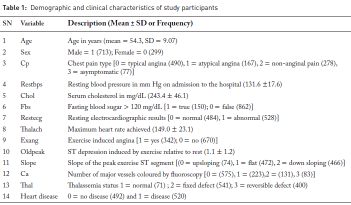
To illustrate the regression concepts, we used a widely cited heart disease prediction dataset from the Kaggle Repository.(ll) The dataset includes demographic, clinical, and diagnostic data as described in Table 1.

 

LINEAR REGRESSION

Simple linear regression

Simple or univariable linear regression is used to estimate the effect of one explanatory variable on the continuous outcome variable. In our example, the impact of each explanatory variable on cholesterol level (outcome variable) was examined. Simple linear regression models generate a beta or regression coefficient which represents the expected change in Y (outcome variable) for a one-unit increase in X (explanatory variable). A positive beta coefficient indicates a direct relationship between the explanatory

variable and the outcome, a negative coefficient indicates an inverse relationship, and a coefficient of zero suggests no linear relationship. The constant value (β₀) is also commonly provided by statistical packages and is interpreted as the expected value of Ywhen X = 0. It is important to note that the intercept is often not clinically meaningful, especially when "zero" is not a realistic or interpretable value of the explanatory variable.

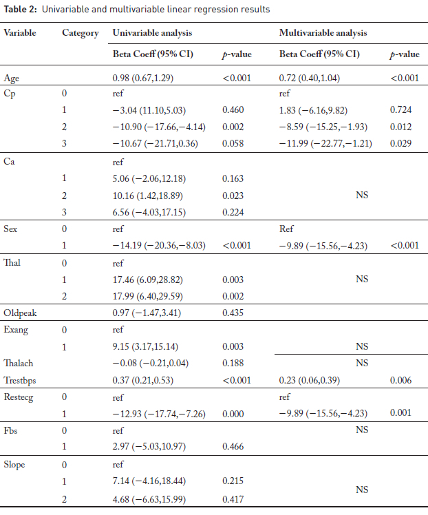
In the univariable model presented here, age was significantly associated with cholesterol level (Table 2). Each additional year of age was associated with an estimated 0.98 mg/dL increase in cholesterol level (95% CI: 0.67,1.29; p < 0.001). The confidence interval (CI) and p-value are key outputs for interpreting regression coefficients. The 95% confidence interval reflects the precision of the estimated effect. The narrower the interval, the more precise the estimate. The CI also indicates statistical significance if it excludes zero. P-values below 0.05 suggest the relationship is unlikely due to chance (statistically significant). The regression model also estimates the coefficient of determination (R²)and the F-statistic. The R² value measures the proportion of variance in the outcome variable explained by the explanatory variable. In the univariable model (Table 2), the relationship between cholesterol levels and age yielded an of 0.037, indicating that approximately 3.7% of the variability in cholesterol levels is explained by age. Low values are common in clinical research due to the multifactorial nature of health outcomes.(12) Despite the low R², the model is statistically significant (F-statistic (1, 1010) = 38.96, p < 0.001), suggesting that age is a significant explanatory variable of cholesterol levels in this dataset. Linear regression assumes that the outcome variable is linearly related to the predictors and that residuals are normally distributed, independent, and homosce-dastic.(7) These assumptions were valid for this dataset.

Multiple linear regression

Multiple (Multivariable) linear regression allows the inclusion of additional explanatory variables to adjust for confounding. In multiple linear regression, the goal is not only to model the outcome variable Y, but also to identify which explanatory variables contribute most significantly to explaining the variability in Y. In the multivariable linear regression model presented here, we estimated the independent effect of each variable on cholesterol levels while adjusting for the influence of other covariates.

Multivariable linear regression identified age, sex, chest pain type (cp), resting blood pressure (trestbps), and resting ECG results (restecg) as significant factors associated with cholesterol levels (Table 2). The interpretation of the effects in the above model follows that of simple linear regression; however, the researcher needs to acknowledge the adjustment of other variables in the model. For instance, one would state that a one-year increase in age significantly increases the cholesterol level by 0.72 (95% CI: 0.40, 1.04; p <0.001) on average, adjusting for other explanatory variables in the model. Similarly, the model shows that after adjusting for other variables, higher resting blood pressure was associated with higher cholesterol, while being male and having abnormal ECG or certain chest pain types were associated with lower cholesterol levels.

Multicollinearity among predictor variables can be checked using the variance inflation factor (VIF), as high multicollinearity can inflate the standard errors of the regression coefficients, leading to unstable estimates and reducing the model's interpretability. Although there are no universally accepted rules for determining when a VIF is excessively high, commonly used guidelines suggest that VIF values of 5 or 10 and above may indicate sufficiently strong collinearity to warrant corrective action.(15)

 

LOGISTIC REGRESSION

Simple logistic regression

Simple logistic regression is used to model the log odds of an outcome with one explanatory variable. The regression/ Beta coefficient reflects the change in the log odds of the outcome for a one-unit increase in the explanatory variable, while the intercept or constant represents the log odds of the outcome when X = 0.

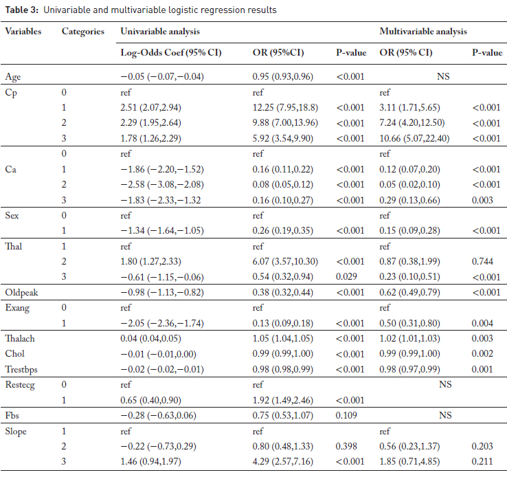
In the logistic regression example presented here, we investigated factors associated with the presence of heart disease using both univariable and multivariable logistic regression models, as carried out in linear regression analyses. When looking at the association of age with heart disease, the coefficient for age is -0.055, indicating that for each additional year of age, the log odds of having heart disease decrease by 0.055.

Although this is a valid interpretation, log odds are not easily interpretable for many clinical researchers and are not conventionally presented. For this reason, it is common practice to express the regression coefficient in its exponential form, yielding the odds ratio (OR). The OR compares the odds (likelihood) of the outcome per unit change in the explanatory variable, which can be either continuous or categorical. An OR of 1 indicates no association between the predictor and the outcome. An OR greater than 1 suggests increased odds of the outcome, while an OR less than 1 indicates decreased odds.(7) For example, the OR corresponding to the age coefficient of -0.055 is calculated as e^-0055 = 0.946, indicating that each additional year of age is associated with a 5.4% decrease in the odds of heart disease.

For categorical variables such as sex (Table 3), where male is coded as "1" and female as "0", the odds ratio comparing males to females is e^-1344 = 0.266. This can also be interpreted as a per cent change using the formula: % change = 100 X (OR - 1)%. Thus, the odds of having heart disease are approximately 73.4% lower in males than in females.

As with linear regression, a p-value below 0.05 suggests the relationship is unlikely to be due to chance; furthermore, the 95% confidence interval indicates significance if it excludes one.

Multiple logistic regression

The simple logistic regression model can be extended to include multiple explanatory variables, resulting in a multi-variable logistic regression model where several explanatory variables are included in the model, and each Beta coefficient represents the change in the log odds of the outcome associated with a one-unit increase in the corresponding variable, holding all other variables constant.

In the example shown in Table 3, 10 variables were retained in the multivariable logistic regression model based on the purposeful variable selection method. Specifically, patients with asymptomatic chest pain (cp = 3) had approximately 10.7-fold higher odds of developing heart disease compared to those with typical angina (reference group) (OR = 10.66, 95% CI: 5.07-22.40). Similarly, atypical angina (cp = 2) also showed a strong positive association with heart disease (OR = 7.24), while being male was associated with significantly lower odds of heart disease (OR = 0.15, 95% CI: 0.09-0.28). Variables such as slope were not statistically significant (p > 0.05), indicating no strong independent effect in the presence of other explanatory variables.

Like linear regression, the multivariable model showed good fit to the data, with a highly significant likelihood ratio test (χ² (16) = 773.88, p < 0.001) and a pseudo R² of 0.55.

 

CONCLUSION

Regression models are powerful tools in clinical research that enable relationships between outcome and explanatory variables. This paper underscores the importance of selecting appropriate models based on the nature of the outcome variable, while ensuring that model assumptions hold, and correctly interpreting results such as beta coefficients and odds ratios. Using linear and logistic regression examples, including univariable and multivariable analyses, we demonstrated how these models can be used to model continuous and binary outcomes while accounting for confounding variables.

 

REFERENCES

1. Del Águila MR, Benítez-Parejo N. Simple linear and multivariate regression models. Allergol Immunopathol (Madr). 2011; 39(3):159-173.         [ Links ]

2. Nunez E, Steyerberg EW, Nunez J. Regression modeling strategies. Rev Esp Cardiol (Engl Ed). 2011; 64(6):501-507.         [ Links ]

3. Sheather S. A modern approach to regression with R. Berlin: Springer Science & Business Media; 2009.         [ Links ]

4. Worster A, Fan J, Ismaila A. Understanding linear and logistic regression analyses. Can J Emerg Med. 2007; 9(2):111-113.         [ Links ]

5. Castro HM, Ferreira JC. Linear and logistic regression models: when to use and how to interpret them? SciELO Brasil; 2022.         [ Links ]

6. Gail M, Krickeberg K, Samet J, Tsiatis A, Wong W. Statistics for biology and health. Berlin: Springer; 2007.         [ Links ]

7. Vittinghoff E, Glidden DV, Shiboski SC, McCulloch CE. Regression methods in biostatistics: linear, logistic, survival, and repeated measures models. Berlin: Springer Science & Business Media; 2012.         [ Links ]

8. Zhu C, Blizzard C, Stankovich J, Wills K, Hosmer DW. Be wary of using Poisson regression to estimate risk and relative risk. Biostat Biom Open Access J. 2018; 4(5):555649.         [ Links ]

9. Andrade C. Understanding relative risk, odds ratio, and related terms: as simple as it can get. J Clin Psychiatry. 2015; 76(7):21865.         [ Links ]

10. Achilonu OJ, Fabian J, Musenge E. Modeling long-term graft survival with time-varying covariate effects: an application to a single kidney transplant centre in Johannesburg, South Africa. Front Public Health. 2019; 7:201.         [ Links ]

11. Ali MM, Paul BK, Ahmed K, et al. Heart disease prediction using supervised machine learning algorithms: performance analysis and comparison. Comput Biol Med. 2021; 136:104672.         [ Links ]

12. Schober P, Boer C, Schwarte LA. Correlation coefficients: appropriate use and interpretation. Anesth Analg. 2018; 126(5):1763-1768.         [ Links ]

13. Bursac Z, Gauss CH, Williams DK, Hosmer DW. Purposeful selection of variables in logistic regression. Source Code Biol Med. 2008; 3:1-8.         [ Links ]

14. Hosmer DW, Lemeshow S, May S. Applied survival analysis: regression modeling of time-to-event data (Wiley series in probability and statistics). Hoboken, NJ: Wiley-Interscience; 2008: 60.         [ Links ]

15. Craney TA, Surles JG. Model-dependent variance inflation factor cutoff values. Qual Eng. 2002; 14(3):391-403.         [ Links ]

 

 

Correspondence:
Okechinyere Achilonu
okechinyere.achilonu@wits.ac.za