RESEARCH ARTICLE
https://doi.org/10.18489/sacj.v36i2.20099

 

Predicting the performance of ORB-SLAM3 on embedded platforms

 

 

Jacques Matthee^I; Kenneth R. Uren^I; George van Schoor^II; Corné van Daalen^III

^ISchool of Electrical, Electronic and Computer Engineering, North-West University. Email: Jacques Matthee - j.matthee97@gmail.com; Kenneth R. Uren - kenny.uren@nwu.ac.za (corresponding)
^IIUnit for Energy and Technology Systems, North-West University. Email: George van Schoor - george.vanschoor@nwu.ac.za
^IIIDepartment of Electrical and Electronic Engineering, Stellenbosch University. Email: Corné van Daalen - cvdaalen@sun.ac.za

 

 

---

ABSTRACT

Simultaneous Localization and Mapping (SLAM) is a crucial component to the push towards full autonomy of robotic systems, yet it is computationally expensive and can rarely achieve real-time execution speeds on embedded platforms. Therefore, a need exists to evaluate the performance of SLAM algorithms in practical embedded environments - this paper addresses this need by creating prediction models to estimate the performance that ORB-SLAM3 can achieve on embedded platforms. The paper uses three embedded platforms: Nvidia Jetson TX2, Raspberry Pi 3B+ and the Raspberry Pi 4B, to generate a dataset that is used in training and testing performance prediction models. The process of profiling ORB-SLAM3 aids in the selection of inputs to the prediction model as well as benchmarking the embedded platforms' performances by using PassMark. The EuRoC micro aerial vehicle (MAV) dataset is used to generate the average tracking time that the embedded platforms can achieve when executing ORB-SLAM3, which is the target of the prediction model. The best-performing model has the following results 2.84%, 3.93%, and 0.95 for MAE, RMSE and R² score respectively. The results show the feasibility of predicting the performance that SLAM applications can achieve on embedded platforms.

Categories • Computer system organization ~ Real-time systems ~ Embedded and cyber-physical sytems

Keywords: Monocular-Inertial SLAM, ORB-SLAM3, Embedded platform, Nvidia Jetson TX2, Raspberry Pi

---

 

 

1 INTRODUCTION

Simultaneous Localization and Mapping (SLAM) is the process where a robot or vehicle concurrently creates a representation of its environment while determining its position within the environment. SLAM presents two primary challenges: To create an accurate map of the environment, the robot needs to have an accurate localisation; and to accurately localise a robot in an environment, an accurate representation of the environment is needed (Kumiawan et al., 2016). SLAM implementations consist of four major algorithmic components: landmark extraction, data association, state estimation, and state and landmark update. Each component has multiple solutions, depending on the environment, sensors used, and the platform it is implemented on; thus, SLAM is a diverse topic which is often associated with high computational expense. There are algorithms (Oriented FAST and Rotated BRIEF (ORB) (Rublee et al., 2011), Scale-Invariant Feature Transform (SIFT) (Lowe, 2004), Speeded-up Robust Features (SURF) (Bay et al., 2008)) that extract features from the environment to be used with other algorithms, such as pose (position and orientation) graph optimisation or bundle adjustment (BA) to estimate the pose and generate a map of the environment.

Eyvazpour et al. (2022) and Barros et al. (2022) illustrate the extensive variety of approaches to SLAM, reflecting the complexity and diversity of solutions in the field. Barros et al. (2022) highlight that the main challenges with current SLAM techniques include algorithmic robustness, computational resource usage, and the ability to understand real-world dynamic environments. In contrast, Eyvazpour et al. (2022) focus on the performance differences among various SLAM techniques across embedded platforms, emphasising that selecting an appropriate hardware platform for SLAM implementation requires careful consideration of factors such as cost, power consumption, computational power, and the specific application.

There is a practical need for SLAM to be implemented on mobile platforms for real-world scenarios such as search-and-rescue operations, military reconnaissance and attack, and automatic exploration of areas. All these endeavours can be autonomously performed by SLAM. The building blocks needed to implement SLAM are: sensors, actuators, processors, and algorithms. The processors and algorithms control the flow of information between the sensors and the actuators. Different sensors can be used in SLAM implementations such as: sonar (Kleeman, 2003), LiDAR (Kohlbrecher et al., 2011), and various types of camera configurations. The type of robotic platform that is used highly influences the choice of sensors. The most significant contributors in deciding what system and sensors to use in SLAM are the cost and the computational load of the required calculations. Sensors such as LiDAR provide accurate results, but an inexpensive camera can achieve similar results depending on the environment.

Visual SLAM (VSLAM) has gained popularity over the past years as it can provide a very detailed representation of the environment in a 3D space, with the disadvantage of being more computationally expensive due to a large amount of information within an image (Chen et al., 2018). However, due to the high level of detail, VSLAM can be used for autonomous navigation and mapping applications. VSLAM can be divided into three categories: monocular, stereo, and RGB-d, according to the camera types used (Taketomi et al., 2017). Monocular SLAM uses a single camera as input, thus being the least computationally and physically expensive VSLAM method. However, monocular SLAM has the disadvantage of the scale ambiguity problem, as scale cannot be determined from a single camera. Therefore, VSLAM has been expanded into visual-inertial SLAM (VISLAM), where visual and inertial data are used to obtain more stable estimation results or, in the case of monocular SLAM, to remove the scale ambiguity problem (Taketomi et al., 2017).

Abouzahir et al. (2017) showed that there is a large performance difference when executing certain SLAM algorithms on an embedded platform versus a high-end desktop computer. The execution performance achieved by the desktop is 1.8, 6.4 and 2.2 times faster for FastSLAM2.0 (Montemerlo et al., 2003), ORBSLAM (Mur-Artal et al., 2015) and RatSLAM (Milford et al., 2004) respectively. Nardi et al. (2015) created SLAMBench 1.0, which provided a portable but untuned KinectFusion (Newcombe et al., 2011) implementation of SLAM in C++ OpenMP, Cuda, and OpenCL. From a performance comparison of KinectFusion on a high-end computer and embedded devices, it is found that the high-end machine can achieve a frame rate of 135 frames per second (FPS), while the best performing embedded device is the Nvidia TK1 with a frame rate of 22 FPS. The TK1's performance is considerably lower than that of the high-end device, but the authors asserted that this performance could almost be classified as real-time. Peng et al. (2020) evaluated two popular visual SLAM techniques, ORBSLAM2 (Mur-Artal & Tardos, 2017) and OpenVSLAM (Sumikura et al., 2019), on the 3 Nvidia Jetson platforms. It is found that the Nvidia Jetson TX2 could run both visual SLAM algorithms within their real-time constraints. An alternative ORB-SLAM2 algorithm that is modified to use the power of a GPU is also investigated. The GPU-accelerated ORB-SLAM2 algorithm increased the performance by 10 FPS while consuming less power than the original algorithm. This shows that although satisfactory results can be obtained using SLAM on high-end machines, there is still a performance gap when using them on embedded devices due to their hardware constraints.

There are three notable benchmarking tools for SLAM: SLAM Hive (Liu et al., 2024), GSLAM (Zhao et al., 2019), and SLAMBench 3.0 (Bujanca et al., 2019). These software frameworks enable researchers and developers to evaluate a wide range of SLAM techniques across various datasets. They focus on critical performance metrics such as accuracy and speed, providing a consistent basis for comparing the robustness and efficiency of different SLAM algorithms in diverse environments. However, these benchmarking tools are not capable of estimating the performance of SLAM algorithms on specific hardware platforms.

This paper makes a two-fold contribution: Profiling ORB-SLAM3 on the Nvidia Jetson TX2 to identify the execution bottlenecks, and creating a model capable of estimating the performance that ORB-SLAM3 can achieve on embedded platforms.

The paper is organised as follows: Section 2 details the hardware and software used within the study, along with the initial implementation. Section 3 profiles the software to identify its bottleneck impact on the hardware. Section 4 discusses the experimental design used to create a model that can estimate the performance of ORB-SLAM3 on embedded platforms. Section 5 provides and discusses the results of the modelling process. Section 6 concludes the study.

 

2 HARDWARE AND SOFTWARE IMPLEMENTATION

2.1 Hardware - Embedded platforms

Three embedded platforms were selected for experimentation: the Nvidia Jetson TX2, Raspberry Pi 3B+, and Raspberry Pi 4B. The Jetson TX2 features a heterogeneous multi-processing environment with two CPU clusters: a dual-core Nvidia Denver 2, optimised for single-threaded performance, and a quad-core ARM Cortex-A57, suited for multi-threaded tasks. In contrast, the Raspberry Pi 3B+ and 4B are equipped with quad-core ARM Cortex-A53 and Cortex-A72 CPUs, respectively.

Table 1 compares these CPUs. The Denver 2, with its superscalar width of seven in Dynamic Code Optimization (DCO) mode, offers the highest potential instruction execution per cycle, surpassing the Cortex-A53, A57, and A72. While the A72 and A57 are "out-of-order" processors that handle code dependencies more effectively, the "in-order" Denver 2 addresses these challenges through DCO.

 

 

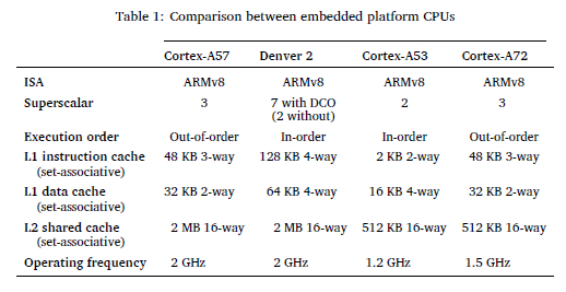
Additionally, the Denver 2's larger L1 cache and higher associativity reduce miss rates but increase access times, whereas the Cortex-A53 experiences more conflict misses with quicker access times. Overall, the Denver 2 provides a balance of lower miss rates with a higher miss penalty.

The hardware listed in Table 1 was selected for this study due to their status as some of the most powerful and widely used embedded platforms available today. Each platform features multi-core CPUs, facilitating parallel processing. Additionally, the Jetson TX2 includes a robust GPU that can be leveraged for enhanced performance. ORB-SLAM3 was executed on all three platforms, and performance metrics captured from which the performance of ORB-SLAM3 on similar embedded systems could be estimated.

2.2 Software - ORB-SLAM3

ORB-SLAM is a highly robust feature-based monocular SLAM system that can operate in real-time in small and large indoor and outdoor environments (Mur-Artal et al., 2015). It also includes loop closing, relocalisation, and complete automatic initialisation. ORB-SLAM uses the same features for all SLAM tasks such as tracking, mapping, relocalisation, and loop closing. The point and keyframes of ORB-SLAM are selected using survival of the fittest, leading to reconstruction with excellent robustness and compact map generation that only grows if the scene changes. ORB-SLAM uses ORB features as a feature extractor, which allows for real-time performance while providing good invariance to changes in viewpoints and illumination differences (Rublee et al., 2011).

ORB-SLAM is written to use three threads that run in parallel: tracking, local mapping, and loop closing. The tracking thread is responsible for localising the camera with every frame and deciding when to insert a new keyframe. The local mapping thread is responsible for processing any new keyframes and performs local BA to achieve optimal reconstruction of the camera pose. The loop closing thread searches for loops with every new keyframe.

ORB-SLAM2 (Mur-Artal & Tardos, 2017) was released two years after ORB-SLAM, and expanded functionality beyond monocular SLAM into stereo and RGB-D SLAM. Another two years later, ORB-SLAM3 (Campos et al., 2021) was released, which is the first system to perform visual, visual-inertial, and multi-map SLAM with monocular, stereo, and RGB-D cameras, using the pin-hole and fisheye lens models. The fact that ORB-SLAM3 allows the user to use different SLAM types, with different sensor input types and various camera models, makes it an ideal SLAM algorithm to investigate. ORB-SLAM3 is a state-of-the-art algorithm extensively used in the research community for visual SLAM tasks (Abouzahir et al., 2017; Barros et al., 2022; Eyvazpour et al., 2022; Peng et al., 2020; Ragot et al., 2019). It is known for its robust performance and versatility across various applications. ORB-SLAM3 leverages ORB (Oriented FAST and Rotated BRIEF) features to deliver accurate and efficient SLAM capabilities, making it a popular choice for research and practical implementations in the field.

The primary objective of this study is to predict the performance of ORB-SLAM3 on an embedded platform, with a specific focus on execution time. In mission-critical applications such as search and rescue, reconnaissance, and attack missions, SLAM applications are only valuable if they can operate in real time.

The way ORB-SLAM3 is written, the tracking thread is the main thread of execution, and if the main thread is stalled or slow, the overall performance of ORB-SLAM3 will be slow. The important performance metric, therefore, is the tracking thread execution time. The objective of the model created in this study is therefore to predict the mean tracking time of ORB-SLAM3 on an embedded platform.

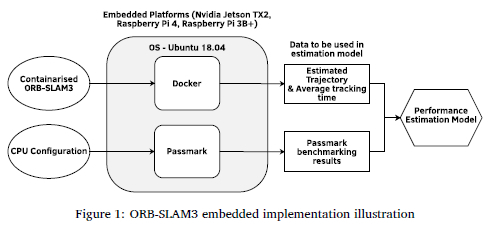
2.3 Implementation

Ubuntu 18.04 was installed on all embedded platforms, along with Docker (Docker, 2018) and Passmark (PassMark, 2024). Passmark was utilised to benchmark CPU performance, providing input for the estimation models. Docker enabled the execution of a containerised version of ORB-SLAM3 on these platforms. The results from Passmark benchmarking and the containerised ORB-SLAM3 were used to develop a performance estimation model. Figure 1 illustrates the software setup on the embedded platforms and how the software was used to generate training and testing data for the performance estimation model.

 

 

3 PERFORMANCE PROFILING

3.1 ORB-SLAM3 profiling

ARM MAP (ARM, 2024b), which was employed in this study, can expose performance problems and bottlenecks by measuring the computation over the time of an application, showing the thread activity, and providing access to the CPU performance measuring unit (PMU) to count the performance events. Due to licensing constraints, profiling was only done on the ARM Cortex A57 CPU of the Nvidia Jetson TX2.

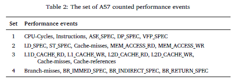
Profiling aims to identify bottlenecks in ORB-SLAM3 on the Nvidia Jetson TX2 and to determine program characteristics such as total instructions executed, instruction mix, and cache performance. The total instructions executed show how many instructions were completed during program execution. Instructions are commonly divided into four groups: arithmetic, load, store, and branch. The combination of instruction types is called instruction mix and indicates what type of instructions are dominant in the program. Cache performance indicates how many times the cache was accessed and what the cache miss ratio was. These program characteristics can be used to aid in the selection of inputs into the prediction model.

Since the ARM A57 CPU has only 6 hardware counters available, the events were measured in four different sets as listed in Table 2 during four separate executions of ORB-SLAM3. Each group was linked to a specific instruction type, such as arithmetic instructions, load and store instructions, cache performance, and branch performance for sets 1-4 listed in Table 2. For the event description, please refer to ARM (2024a).

 

 

Using ARM MAP to profile ORB-SLAM3, it was identified that the CPU is constantly working and not waiting for any other input, indicating that ORB-SLAM3 is compute intensive on the Nvidia Jetson TX2.

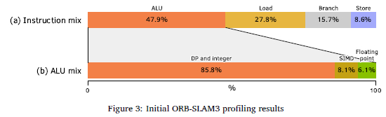
By analysing the function call stack in Figure 2, the FAST function of the OpenCV library was found to be the most time-consuming. This function is called within ORB-SLAM3's ComputeKeypointsOctTree function, which forms part of the ORBextractorOperator.

 

 

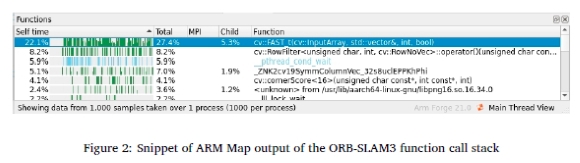
Figure 3(a) shows that ORB-SLAM3 is dominated by arithmetic logic unit (ALU) instructions, followed by load instructions. Figure 3(b) shows that the ALU instructions were dominated by data processing and integer math instructions with relatively few SIMD instructions, which indicates that ORB-SLAM3 was poorly optimised to use single instruction multiple data SIMD instructions on the Nvidia Jetson TX2. The high amount of load instructions was due to the sequence images loaded into the cache hierarchy, for processing by the CPU.

 

 

No modifications were made to the ORB-SLAM3 source code to enhance efficiency. However, there was potential for performance improvement on the Nvidia Jetson TX2 by modifying the source code to utilise the GPU's CUDA cores.

 

4 EXPERIMENTAL DESIGN

The previous sections described the hardware characteristics of the embedded platforms used in the study and how software such as ORB-SLAM3 executed on them. This section describes the creation of a prediction model to estimate the performance of ORB-SLAM3 on embedded platforms.

4.1 Model inputs and outputs

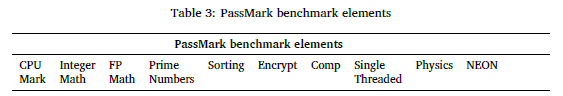
Since ORB-SLAM3 is CPU-Bounded on embedded platforms, the CPU characteristics were used as inputs to the model. One method to characterise a CPU is using a benchmark program such as PassMark which is a collection of CPU stress tests that executes on the CPU to determine its performance. Table 3 shows the categories that are tested by the PassMark benchmark. The CPU mark is an overall score that combines all the other categories. The rest of the categories are individual benchmark test scores where specific programs are executed to test the CPU performance in a specific category. All tests were done with multi-threading except for the CPU single-threaded test. These benchmark scores were investigated and reduced to be used as inputs to the prediction model.

 

 

Since the FAST algorithm forms part of the tracking thread and is the bottleneck of ORB-SLAM3, the maximum performance that ORB-SLAM3 can achieve on an embedded platform is determined by the speed at which the platform can execute the tracking thread. Thus the prediction model predicts the average tracking time that ORB-SLAM3 can achieve on a given platform.

4.2 Dataset generation for modelling

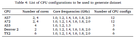
With the inputs and output defined, data had to be gathered to train and test the model. The model output was generated by executing the 11 EuRoC MAV sequences on the embedded platforms. The study had access to three embedded platforms with a total of four different CPUs: the Nvidia Jetson TX2 (Denver 2 and A57 CPUs), the Raspberry Pi 3B+ (A53) and the Raspberry Pi 4B (A72). If all 11 sequences were executed on the four different CPUs, the dataset would only contain 44 data pairs, which could limit the prediction model's performance. Thus the number of available CPUs was artificially increased by setting up different CPU configurations to generate enough data pairs for the model creation.

Generating the different CPU configurations was achieved through over-clocking and under-clocking the different CPU cores and limiting the number of available CPU cores.

Table 4 shows the 39 CPU configurations that were used to generate the prediction model dataset, by varying the number of CPU cores and CPU core frequencies.

 

 

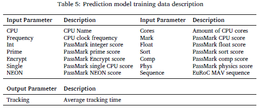
By executing the 11 EuRoC MAV sequences on the 39 available CPU configurations, the data set will have 429 data pairs. The prediction model training data comprises 15 parameters as described in Table 5. It constitutes the CPU name, clock frequency, PassMark benchmarking results, the executed sequence as 14 model inputs and the average tracking time that the specific CPU configuration achieved while executing ORB-SLAM3 as model output.

 

 

4.3 Data collection and pre-processing

Two separate steps were followed in collecting data: benchmarking the CPU configuration and executing ORB-SLAM3 with the 11 EuRoC MAV sequences. Once the CPU frequency was set, the PassMark benchmark was executed to characterise the performance of the CPU configuration. Afterwards, the 11 EuRoC MAV sequences were executed on the platform using a created Docker container that containerised ORB-SLAM3 for the embedded platforms. The results of the PassMark benchmarking and ORB-SLAM3 execution are combined in a table format shown in Table 5. Figure 4 shows the procedure that was followed to generate the necessary dataset. The data used for training the models can be accessed at https://figshare.com/s/ec2a3faca0f1311ed7dd.

 

 

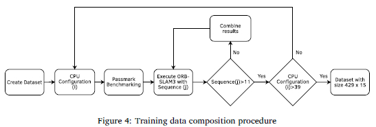
Out of the 15 parameters in the dataset, 14 are chosen as inputs, and the last parameter was designated output of the model, i.e. the average tracking time that ORB-SLAM3 achieved for the different EuRoC MAV sequences on the different CPU configurations. It is important to note that the 14 parameters were immediately reduced to 13, as it was decided to always include the EuRoC MAV sequence as an input to ensure that the model would have 429 unique data pairs. If the EuRoC MAV sequence had been left out, there would have been only 39 unique entries in the dataset. To further reduce the complexity of the prediction model, two feature selection methods were used: the correlation between the target value and the remaining inputs and a user-selection method guided by profiling as described in the previous sections.

4.4 Model creation

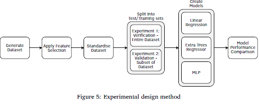
After the dataset has been generated, the prediction models could be created. Different prediction models were created and evaluated to determine which one performed the best. With the dataset created, feature selection was applied to it to select the inputs that have a performance impact on the average tracking time on embedded platforms. The feature selection process was guided by calculating the correlation between the target and all the inputs and by the knowledge gained through the literature study and the profiling of ORB-SLAM3. After the feature selection process, the dataset was standardised using Python's StandardScalar module to ensure that the dataset has zero mean and unit variance.

Two experiments were conducted, Experiment 1 for verification and Experiment 2 for validation. The only difference between the two experiments was the data pairs used to train and test the models. Experiment 1 used the entire dataset with a ratio of 75:25 split ratio for training and testing. Experiment 2 was trained on only a subset of the dataset to see how the models perform on an unseen embedded platform. The subset of training data included the data pairs of the A72, A53, and Denver 2 CPUs, with the test data being the data from the A57 CPU. The data from the TX2 CPU were removed as it combined the A72 and A57 CPUs performances. This dataset constituted 363 data pairs, of which 231 pairs were used for training and 132 for testing, effectively creating a training test set with a 63:37 split ratio. If the model could achieve adequate performance for an unseen embedded platform, the model would be validated.

Three modelling techniques were used: a simple Linear Regression model, an ExtraTrees Regressor, and a multi-layer perceptron model, MLP. Linear Regression offers a straightforward and interpretable baseline, which allowed the assessing of whether a simple modelling technique could address the problem. The ExtraTrees Regressor was selected for its robustness and accuracy, combining multiple decision trees to mitigate overfitting and improve generalisation. The Multi-Layer Perceptron (MLP) was chosen for its capability to capture complex, non-linear patterns. These models were created using sklearn.linear_model.LinearRegression, sklearn.ensemble.ExtraTreesRegressor, and sklearn.neural_network.MLPRegressor. The Linear Regression and ExtraTrees models used default settings, while the MLP model was configured with random_state = 42, hidden_layer_sizes = 200, and max_iter = 10000. Together, these models provided a comprehensive evaluation, ranging from basic to advanced approaches. The last step in the model creation process was to compare the performances of the different models. Figure 5 shows the steps of the experimental design.

 

 

The performance metrics measured included the mean absolute error (MAE), root mean square error (RMSE), and the coefficient of determination, R².

Table 6 shows the performance metrics criteria that the models had to achieve for verification and validation.

 

 

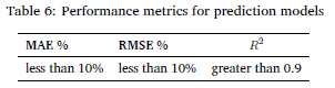
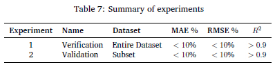
Table 7 summarises the two experiments with their names and their performance criteria.

 

 

5 RESULTS AND DISCUSSION

For verification, the entire dataset was used for training and testing, whereas for validation, a CPU was removed from the dataset to see how the models would perform for unseen CPUs.

5.1 Experiment 1: Verification

With the dataset created, the feature selection method had to be applied to the data to determine what data fields would be used as input for the prediction models. Firstly, the correlation between all the inputs of the dataset were correlated to the target of the model, which was the average tracking time that the embedded platforms achieved during the execution of ORB-SLAMS. The inputs with the highest correlation to the target were selected as inputs to the model. Table 8 shows the top five correlation scores with respect to average tracking time for different model parameters.

 

 

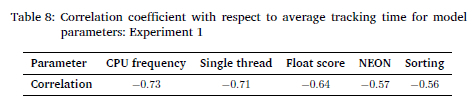
As expected, the most significant correlation coefficient belongs to the CPU frequency, as higher clock frequencies usually mean applications can execute at faster speeds. The second most significant contributor is the Single Threaded CPU score of PassMark.

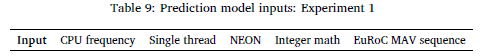
The appropriate inputs of the models were determined by combining the results from the correlation coefficients and the knowledge gained during Experiment 3.1. From the PassMark category results, the following inputs were chosen: Single CPU score, Neon Score and integer score. The Single CPU score was chosen as the tracking thread only executes on a single core and has the second-highest correlation coefficient. The Neon score was also selected as the FAST algorithm executes with NEON instructions and contains 19.93% NEON instructions. The correlation coefficient also showed that the NEON score strongly correlated with the model's target. The integer score was the last input, as it is the largest portion of executed instructions during the FAST algorithm, with 3.71%. Table 9 summarises the inputs that were used to create the models.

 

 

Python is used to create the prediction models. The data were first standardised using Python's StandardScalar module to ensure that the dataset has zero mean and unit variance. The dataset was also split into a training and test set with a ratio of 75:25 to be used for the models' verification.

Different models were created to see what model would provide the best results. Modelling techniques such as linear regression, ExtraTrees and a simple MLP regressor were used to create the models. All the models were used from the Scikit-learn library, including LinearRegression from the linear model module (Scikit-learn, 2024b), ExtraTreesRegressor from the ensemble module (Scikit-learn, 2024a), and the MLPRegressor from the neural network module (Scikit-learn, 2024c).

The linear regression model is an ordinary least squares linear regression model with all the default Python settings. This model was chosen for its simplicity. The ExtraTrees ensemble methods were chosen as they provide better performance. They are typically made up of more than one model, and the models learn from each other and they are known for their robustness (Brownlee, 2020), the default settings were also used. The MLP regressor neural network was chosen as it has the ability to learn non-linear relationships in the dataset. The hidden layer size was increased from 100 to 200, and the max iterations to 20000 to allow for convergence.

Table 10 shows the performance of the prediction models.

 

 

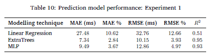
The ExtraTrees model is the best performing model with an MAE and RMSE percentage of 2.84% and 3.93% and a R² score of 0.95. The low MAE and RMSE percentages indicate that the model can make accurate predictions with a small relative error. Both the MAE and RMSE percentages were calculated by dividing their respective values by the range of the target training data multiplied by 100. The high R² score shows that the input variables are good predictors for the target variable. The linear regression model has the worst performance, and the MLP regressor has a comparable performance to the ExtraTrees model.

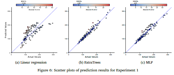
Figures 6(a) to 6(c) show scatter plots for the three prediction models plotting the actual vs. the predicted values. Figure 6(a) shows that the linear regression model is loosely clustered around the diagonal line and cannot make accurate predictions. It should also be noted that it struggles to predict targets with a longer average tracking time accurately. Figures 6(b) and 6(c) are more tightly clustered around the diagonal line, showing their strength in accuracy.

 

 

The performance that the ExtraTrees model achieved verified the model, and confirms the robustness and performance capabilities of ExtraTrees models. However, the models were still trained and tested with all of the embedded platforms. In the next section, the models are validated with some of the embedded platform data not included in the training.

5.2 Experiment 2: Validation

This section validates the models by predicting the average tracking time of ORB-SLAM3 for an embedded platform that is not present in the training set. To achieve this, the dataset had been reduced to only include the data gathered from the Denver 2 CPU, A72 CPU and the A53 CPU. The unknown CPU that was used for testing is the A57 CPU. The TX2 CPU data was removed as it was a combination of the A57 and Denver 2 CPU and could have skewed the results.

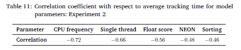
The correlation coefficients were also recalculated, and the results are provided in Table 11. The same top five inputs are present in this training set as with the entire dataset. Since the correlation table did not change, the same inputs were used to create the validation models as used for verification.

 

 

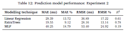
The same three modelling techniques were used, and the performance of the models is displayed in Table 12. The best-performing model is still the ExtraTrees model, with the lowest MAE and RMSE percentages of 9.12% and 13.14%, respectively and a coefficient of determination score of 0.78. Table 12 shows that the linear regression model now performs better than the MLP model. Neither the linear regression nor the MLP model achieved the performance criteria listed in Table 6. Only the ExtraTrees model was able to achieve a MAE% of below 10%. However, it does not meet the RMSE or R² criteria. The RMSE performance is S.14% over the specified value. The R² score of 0.78 is well below the required value of 0.9. The model accuracy can be improved by increasing the training and test set data size by profiling more embedded platforms.

 

 

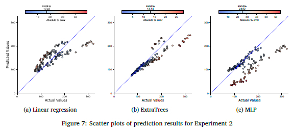
Figures 7(a) to 7(c) show the scatter plots for the three prediction models, plotting the actual vs. the predicted values for Experiment 2. Figure 7(a) reveals that the linear regression model shows poor performance. As with Experiment 1, it predicts longer than actual tracking times. The ExtraTrees model, Figure 7(b), shows the best performance. It can accurately predict the performance of the average tracking time if below 150 ms. Above the latter the error increases. This could mean that the model is over-fitted to that portion of the dataset as there is a denser representation of data in that range. Figure 7(c) shows that the MLP model could accurately predict only a portion of the dataset, with the rest of the predictions forming another distinct pattern.

 

 

Changing the training data influenced the model's results. A contributor to the decrease in performance can be caused by the decrease in training data from S21 data pairs down to 2S1 to train the model with. The MLP had a drastic performance decrease. On the other hand, the linear regression had a similar performance to that of the entire dataset. ExtraTrees is still the best performing model. The experiment validated the approach by creating a model that can predict the performance of ORB-SLAM3 on embedded platforms. However, the models were not able to achieve the required performance, with the ExtraTrees model missing the RMSE criteria with 3.14% and the R² score with 0.12.

 

6 CONCLUSION

The paper showed that the performance that ORB-SLAM3 can achieve on embedded platforms can be predicted. Through profiling and investigation into the execution of the code, different models were created to estimate the performance of ORB-SLAM3 on embedded platforms. The predictive models' target was the average tracking time of ORB-SLAM3, and the inputs to the models were a selection of the PassMark benchmarking results. The models could predict the performance of ORB-SLAM3 with satisfactory results. The ExtraTrees model for Experiment 1, verification, had the best results with 2.84%, 3.93%, 0.95 for the MAE, RMSE and the R² score, respectively. For Experiment 2, validation, the ExtraTrees model was also the best model with the MAE, RMSE, and R² scores 9.12%, 13.14%, 0.78. The paper showed the feasibility of creating a model in estimating the performance of ORB-SLAM3 on embedded platforms. One of the limitations is the number of available embedded platforms to generate the training data, along with the use of only the EuRoC MAV dataset. It should also be noted that the models were trained on CPU architectures of the ARMv8a architecture, so the models will perform poorly on other architectures.

 

References

Abouzahir, M., Elouardi, A., Latif, R., Bouaziz, S., & Tajer, A. (2017). Embedding SLAM algorithms: Has it come of age? Robotics and Autonomous Systems, 100, 14-26. https://doi.org/10.1016/j.robot.2017.10.019        [ Links ]

ARM. (2024a). ARM Cortex-A57 MPCore processor technical reference manual [Accessed: 12 September 2024]. ARM. https://developer.arm.com/documentation/ddi0488/c/CIHBBFEF

ARM. (2024b). Arm MAP: Scalable profiler for server/hpc developers [Accessed: 12 September 2024]. https://www.arm.com/products/development-tools/server-and-hpc/forge/map

Barros, A. M., Michel, M., Moline, Y., Corre, G., & Carrel, F. (2022). A comprehensive survey of visual SLAM algorithms. Robotics, 11(1), 24. https://doi.org/10.3390/robotics11010024        [ Links ]

Bay, H., Ess, A., Tuytelaars, T., & Van Gool, L. (2008). Speeded-up robust features (SURF). Computer Vision and Image Understanding, 110(3), 346-359. https://doi.org/https://doi.org/10.1016/j.cviu.2007.09.014        [ Links ]

Brownlee, J. (2020). Why Use Ensemble Learning? [Accessed: 12 September 2024]. https://machinelearningmastery.com/why-use-ensemble-learning/

Bujanca, M., Gafton, P., Saeedi, S., Nisbet, A., Bodin, B., O'Boyle, M. F., Davison, A. J., Kelly, P. H., Riley, G., Lennox, B., Luján, M., & Furber, S. (2019). Slambench 3.0: Systematic automated reproducible evaluation of SLAM systems for robot vision challenges and scene understanding. 2019 International Conference on Robotics and Automation (ICRA), 6351-6358. https://doi.org/10.1109/ICRA.2019.8794369

Campos, C., Elvira, R., Rodríguez, J. J. G., M. Montiel, J. M., & D. Tardos, J. (2021). ORB-SLAM3: An accurate open-source library for visual, visual-inertial, and multimap SLAM. IEEE Transactions on Robotics, 37(6), 1874-1890. https://doi.org/10.1109/TRO.2021.3075644

Chen, C., Zhu, H., Li, M., & You, S. (2018). A review of visual-inertial simultaneous localization and mapping from filtering-based and optimization-based perspectives. Robotics, 7(3), 45. https://doi.org/10.3390/robotics7030045        [ Links ]

Docker. (2018). Enterprise Application Container Platform - Docker [Accessed: 12 September 2024]. https://www.docker.com/

Eyvazpour, R., Shoaran, M., & Karimian, G. (2022). Hardware implementation of SLAM algorithms: A survey on implementation approaches and platforms. Artificial Intelligence Review, 56(7), 6187-6239. https://doi.org/10.1007/s10462-022-10310-5        [ Links ]

Kleeman, L. (2003). Advanced sonar and odometry error modeling for simultaneous localisation and map building. Proceedings 2003IEEE/RSJ International Conference on Intelligent Robots and Systems (IROS 2003), 1, 699-704. https://doi.org/10.1109/IROS.2003.1250711

Kohlbrecher, S., von Stryk, O., Meyer, J., & Klingauf, U. (2011). A flexible and scalable SLAM system with full 3D motion estimation. 2011 IEEE International Symposium on Safety, Security, and Rescue Robotics, 155-160. https://doi.org/10.1109/SSRR.2011.6106777

Kumiawan, D., Jati, A. N., & Sunarya, U. (2016). A study of 2D indoor localization and mapping using FastSLAM 2.0. 2016 International Conference on Control, Electronics, Renewable Energy and Communications (ICCEREC), 152-156. https://doi.org/10.1109/ICCEREC2016.7814991

Liu, X., Yang, Y., Xu, B., & Schwertfeger, S. (2024). Benchmarking SLAM algorithms in the cloud: The SLAM hive system [Accessed: 22 October 2024]. https://arxiv.org/abs/2406.17586

Lowe, D. G. (2004). Distinctive image features from scale-invariant keypoints. International Journal of Computer Vision, 60, 91-110. https://doi.org/10.1023/B:VISI.0000029664.99615.94        [ Links ]

Milford, M., Wyeth, G., & Prasser, D. (2004). RatSLAM: A hippocampal model for simultaneous localization and mapping. IEEE International Conference on Robotics and Automation, ICRA2004, 1, 403-408. https://doi.org/10.1109/ROBOT.2004.1307183

Montemerlo, M., Thrun, S., Koller, D., Wegbreit, B., et al. (2003). FastSLAM 2.0: An improved particle filtering algorithm for simultaneous localization and mapping that provably converges. IJCAI'03: Proceedings of the 18th international joint conference on Artificial intelligence, 1151-1156. https://dl.acm.org/doi/10.5555/1630659.1630824

Mur-Artal, R., Montiel, J. M. M., & Tardos, J. D. (2015). ORB-SLAM: A versatile and accurate monocular SLAM system. IEEE Transactions on Robotics, 31(5), 1147-1163. https://doi.org/10.1109/TRO.2015.2463671        [ Links ]

Mur-Artal, R., & Tardos, J. D. (2017). ORB-SLAM2: An open-source SLAM system for monocular, stereo, and RGB-D cameras. IEEE Transactions on Robotics, 33(5), 1255-1262. https://doi.org/10.1109/TRO.2017.2705103        [ Links ]

Nardi, L., Bodin, B., Zia, M. Z., Mawer, J., Nisbet, A., Kelly, P. H. J., Davison, A. J., Luján, M., O'Boyle, M. F. P., Riley, G., Topham, N., & Furber, S. (2015). Introducing SLAMBench, a performance and accuracy benchmarking methodology for SLAM. 2015 IEEE International Conference on Robotics and Automation (ICRA), 5783-5790. https://doi.org/10.1109/ICRA.2015.7140009

Newcombe, R. A., Izadi, S., Hilliges, O., Molyneaux, D., Kim, D., Davison, A. J., Kohi, P., Shotton, J., Hodges, S., & Fitzgibbon, A. (2011). KinectFusion: Real-time dense surface mapping and tracking. 2011 10^th IEEE International Symposium on Mixed and Augmented Reality, 127-136. https://doi.org/10.1109/ISMAR.2011.6092378

PassMark. (2024). PassMark performance test - PC benchmark software [Accessed: 12 September 2024].passmark. https://www.passmark.com/products/performancetest/index.php

Peng, T., Zhang, D., Hettiarachchi, D. L., & Loomis, J. (2020). An evaluation of embedded GPU systems for visual SLAM algorithms. Electronic Imaging, 32(6), S25. https://doi.org/10.2352/ISSN.2470-1173.2020.6.IRIACV-325        [ Links ]

Ragot, N., Khemmar, R., Pokala, A., Rossi, R., & Ertaud, J.-Y. (2019). Benchmark of visual SLAM algorithms: ORB-SLAM2 vs RTAB-Map. 2019 Eighth International Conference on Emerging Security Technologies (EST). https://doi.org/10.1109/est.2019.8806213

Rublee, E., Rabaud, V., Konolige, K., & Bradski, G. (2011). ORB: An efficient alternative to SIFT or SURF. 2011 International Conference on Computer Vision, 2564-2571. https://doi.org/10.1109/ICCV.2011.6126544

Scikit-learn. (2024a). sklearn ExtraTreesRegressor [Accessed:12 September 2024]. https://scikit-learn.org/stable/modules/generated/sklearn.ensemble.ExtraTreesRegressor.html

Scikit-learn. (2024b). sklearn LinearRegression [Accessed: 12 September 2024]. https://scikit-learn.org/stable/modules/generated/sklearn.linear_model.LinearRegression.html

Scikit-learn. (2024c). sklearn MLPRegressor [Accessed: 12 September 2024]. https://scikit-learn.org/stable/modules/generated/sklearn.neural_network.MLPRegressor.html

Sumikura, S., Shibuya, M., & Sakurada, K. (2019). OpenVSLAM: A versatile visual SLAM framework. Proceedings of the 27th ACM International Conference on Multimedia, 2292-2295. https://doi.org/10.1145/3343031.3350539

Taketomi, T., Uchiyama, H., & Ikeda, S. (2017). Visual SLAM algorithms: A survey from 2010 to 2016. IPSJ Transactions on Computer Vision and Applications, 9(1), 1-11. https://doi.org/10.1186/s41074-017-0027-2        [ Links ]

Zhao, Y., Xu, S., Bu, S., Jiang, H., & Han, P. (2019). GSLAM: A general SLAM framework and benchmark. 2019IEEE/CVF International Conference on Computer Vision (ICCV), 1110-1120. https://doi.org/10.1109/ICCV.2019.00120

 

 

Received: 2 November 2023
Accepted: 12 September 2024
Online: 11 December 2024