Local Heat Transfer Measurements During Phase Change Processes Using Microscale Heaters

 

 

Jungho Kim

Associate Professor, University of Maryland, Dept. of Mechanical Engineering, College Park, MD 20742

 

 

---

ABSTRACT

Although liquid-vapour phase-change heat transfer processes have been studied for many years, there remain significant questions regarding the mechanisms by which the energy is transferred. The great majority of experimental data to date has been obtained using heater surfaces that were comparable to, or much larger than the scales at which the heat transfer occurs, enabling only average heat transfer rates and temperatures over the entire heated surface to be obtained. Little experimental data is available regarding the local heat transfer rates during these processes. Time and space resolved heat transfer measurements can be of great benefit in elucidating heat transfer mechanisms during phase change processes by pinpointing when and where large amounts of heat are removed. This paper describes in detail the development of two technologies to provide these measurements, and examples of their application are given.

---

 

 

Introduction

Local heat transfer measurement techniques can be used to provide much needed information regarding heat transfer mechanisms. The ability to determine when and where heat is transferred during a phase change process and correlating this information with visual observations can be a very powerful tool in investigating heat transfer mechanisms. Perhaps the most prevalent form of local heat transfer measurement to date for both single phase and multiphase studies has been the use of thermochromic liquid crystals (TLC) to measure temperature distributions on surfaces.

TLCs have chiral (twisted) molecular structures and are optically active mixtures of organic chemicals. They show colors by selectively reflecting incident white light. Temperature-sensitive mixtures turn from colorless (black against a black background) to red at a given temperature and, as the temperature is increased, pass through the other colors of the visible spectrum in sequence (orange, yellow, green, blue, violet) before turning colorless (black) again at a higher temperature. The color changes are reversible. TLCs have been used to provide fast response wall temperature information over quite large areas for constant wall heat flux boundary conditions for boiling studies (Bayazit et al.¹, Kenning, et al.²). Usually an electric current is sent through a thin stainless steel sheet, heating it. One side of the sheet is coated with black paint, then sprayed with a thin layer of unencapsulated liquid crystal. Thin polymer coating is then applied to protect the liquid crystal. The phase change heat transfer occurs on the opposite side of the stainless steel sheet. This setup provides a nearly constant heat flux boundary condition. Although most of the visualisations to date have been at low frequencies (30 Hz or below), it is possible to obtain data at frequencies as high as 500 Hz if the stainless steel sheet is thin and unencapsulated TLC is used. The advantages of using liquid crystal thermography are that it is relatively inexpensive and temperatures over large areas can be visualised. The disadvantages are that high frequency response is not possible, and the temperatures response range is somewhat limited (typically 25°C). A similar technique is to use an infrared camera to visualise the temperature distribution on a thin, electrically heated stainless steel sheet painted black (Theofanous et al.³).

Some more recent work measured the local heat flux from a heated, transparent surface using laser interferometry to obtain contours of the microlayer thickness underneath growing vapor bubbles versus time (Fath and Judd⁴ and Koffman and Plesset⁵). The rate of change of the microlayer thickness was related to the wall heat transfer through a simple energy balance. This technique allows measurements within the microlayer to be made, but measurements after bubble departure are not possible.

In this paper, two additional methods of measuring local heat transfer are discussed. The first is a passive technique utilising a diode array that provides the temperature distribution on a surface that is heated. The second is an active technique using microheater arrays that provides heat transfer distribution on surfaces that are held at constant temperature. The application of the second technique to two phase-change processes are described.

 

Diode Array

Arrays of diodes can be used to measure temperature distributions on whatever surfaces they can be constructed, by measuring their forward voltage drop as a function of temperature. In the following example, the diodes are made on a silicon wafer, but the same technique can be applied to diodes constructed on flexible polymer substrates (Sheats et al.⁶). The development of this exciting possibility may allow temperatures to be measured on curved surfaces that are not easily accessible, such as the inside surface of tubes.

Diode array construction

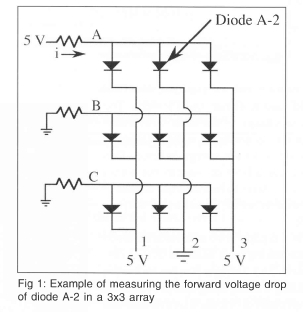
A schematic of how the diodes are connected together is shown on Fig 1 for a 3 X 3 array of diodes. If the voltage drop across diode A-2 is desired, a small current (typically 100 μ A) is sent into row A while the other rows are grounded. Simultaneously, column 2 is grounded while the other columns are set to 5 V. All of the diodes in the array with the exception of A-2 are now either reverse biased (so no current flows through them), or they have no voltage drop across them. The voltage at A is then measured to obtain the forward voltage drop across diode A-2. The voltage drop across the other diodes in the array are obtained by scanning across the array.

 

 

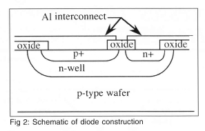
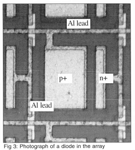
A 32 X 32 p-n junction isolated diode array was built on a p-type wafer using VLSI techniques. A schematic of a single diode is shown on Fig 2. First, a mask was used to create a series of n-wells on the wafer. A second mask was used to implant boron to create regions of p+. A third mask was used to create regions of n+ to make a well contact by diffusing phosphorous. A fourth mask was used to open a contact via the electrical contact to the diode. Finally, a fifth mask was used to interconnect the diodes in the array. Each individual diode is 0.1 mm X 0.1 mm in size, with the entire array being 3.2 mm x 3.2 mm in size. A photograph of a single diode in the array is shown on Fig 3.

 

 

 

 

Many arrays can be made on a single wafer. Once a wafer has been processed, the wafer is diced to obtain the individual chips. These chips are epoxied to a Pin Grid Array (PGA), and connections from the chips to the PGA are made using wire-bonds. For a 32 x 32 diode array, a total of 64 wire bonds need to be made.

Scanning circuitry

A schematic of the circuitry used to scan the diodes in the array and provide signal conditioning is shown in Fig 4. The circuit receives two external signals: a start pulse and a signal from an external clock, both of which enter the counter. The start pulse tells the counter to begin counting, while the external clock is used to set the frequency at which counting occurs. The actual counting frequency is half the clock frequency. Counting frequencies of up to 2.5 MHz are possible with the current circuitry. The signal exiting the counter enters two Erasable Programmable Read Only Memories (EPROM), one for choosing the row and one for choosing the column. Everytime a pulse from the clock enters the EPROMs, they output two 5-bit digital signals corresponding to row and column numbers. In the present configuration, the EPROMs are programmed to increment the column number from 1 to 32 before incrementing the row number. All of the diodes in a particular row are therefore scanned before going on to the next row. The entire array is scanned once every time the circuit receives an external start pulse.

 

 

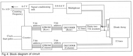
The great advantage of using EPROMs is that any arbitrary subset of diodes can be scanned by simply reprogramming the EPROMs. For example, the EPROMs can be programmed to scan only those diodes underneath a nucleating bubble - since scanning speed stays constant, each diode in this subset of diodes can be scanned at much higher frequencies than if the entire array were scanned.

The measured voltage drops across the diodes are multiplexed into one continuous signal that is typically between 0.8-0.6 V. To take advantage of the resolution of the A/D converter, this signal is sent through a signal conditioning unit that offsets, inverts, and amplifies the signal to match a 0-5 V range.

Data acquisition of the multiplexed signal is performed using an off-the-shelf data acquisition unit (Daqbook 216 from I/O Tech). This unit is capable of scanning a single channel at up to 100 kHz with 16 bits of resolution. Data acquisition is performed with the unit in the 'External Trigger' mode, in other words, a data point is read every time the A/D receives a pulse from the counter.

The current used to sense the voltage drop across the diode must not influence the temperature measurement by heating the diode significantly. The energy dissipated by a typical diode with a 100 mA sensing current is 0.7 W/cm². While this may seem like a large heat flux, it must be remembered that the sensing current is only applied for a very short time (typically 1 ms if scanning occurs at 1 MHz for a 32 x 32 array). An upper bound on the temperature rise of the surface, can be obtained by assuming, that the silicon substrate acts as a semi-infinite solid subjected to a step change in wall heat flux (Incropera and Dewitt⁷):

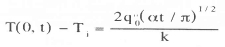
For a wall heat flux of 0. 7 W/cm² and a scanning time of 1 us, the surface temperature rise is just 0.0005 °C, which is well within the uncertainty of the measurement. The actual temperature rise is much lower since only a small portion of the surface is heated.

Calibration

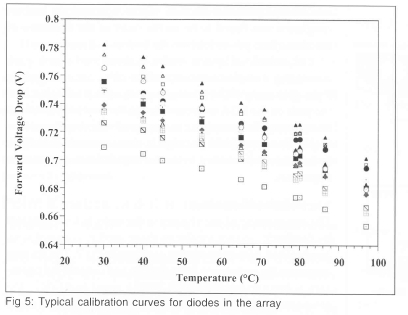
Calibration of the diode array is performed by placing it in a uniform temperature environment, and measuring the forward voltage drop of each diode as a function of temperature. For typical diodes, the forward voltage drop decreases by about 2 mV/°C around room temperature. Typical calibration curves for a few diodes in the array are shown on Fig 5. Measurement of temperatures to within 1°C is easily achievable.

 

 

Summary of ad vantages and disadvantages

There are two advantages of using the diode array to measure temperature distribution. First, measurements can be made at very high speeds, especially if only a portion of the array is scanned. Second, high spatial resolution is possible since diodes can be made as small as a few microns in size. The primary disadvantage is the limited area that can be scanned at present.

 

Microheater Array

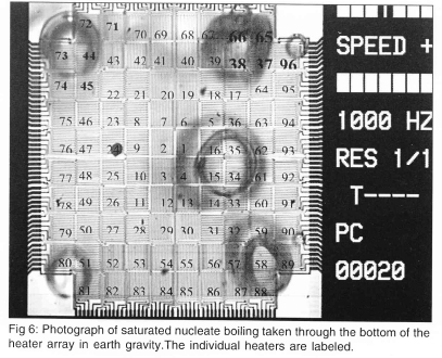
This technique offers the ability to measure heat transfer distributions on an isothermal surface. It can also be operated to provide the temperature distribution on the surface when the surface is heated. The local surface heat flux and temperature measurements are provided by an array of ninety-six platinum resistance heaters deposited on a quartz wafer. A photograph of boiling on this heater array taken through the quartz substrate is shown in Fig 6. Each of the individual heaters is about 0.26 mm X 0.26 mm in size, has a nominal resistance of 1000 W and a nominal temperature coefficient of resistance of 0.002°C^-1. Up to 17 heater arrays can be fabricated simultaneously on a single quartz wafer using VLSI circuit fabrication techniques. Platinum is sputtered onto the entire surface of a 500 μm thick wafer to a thickness of 0.2 μm, a layer of photoresist is deposited and patterned to define the heater geometry, then the platinum from the unmasked areas is removed using an ion mill to form a resistance heater. The platinum lines within each individual heater are 5 μm wide and spaced 5 μm apart. The spacing between each heater in the array varies from 7 μm near the center of the array to typically 40 μm between heaters on the outer edge of the array. Aluminium is then vapor-deposited to a thickness of 1 μm onto the surface, the aluminium power leads are masked off, and the remaining aluminium is removed using a wet chemical etch. A layer of SiO₂ is finally deposited over the heater array to provide the surface with a uniform surface energy. The surface was viewed under an electron microscope, and the surface roughness was found to be on the order of the thickness of the aluminium power leads to the heaters (~1 μm).

 

 

The completed quartz wafer is diced into chips, each containing a single heater array. The chips are mounted on a pin-grid-array (PGA) package using epoxy adhesive, and the pads on the PGA are connected to the power leads of the heater array chip using a conventional wire-bonding technique. The completed package is then mounted in a PGA socket that is connected to the control and data acquisition apparatus.

Electronic feedback loops

The temperature of each heater in the array is kept constant by feedback circuits similar to those used in constant temperature hot-wire anemometry as shown in Fig 7. The op-amp measures the imbalance in the bridge and outputs the necessary voltage to keep the ratio RH/R1 equal to RC/R2. The temperature of the heater is controlled by changing the wiper position of the digital potentiometer. The instantaneous voltage required to keep each heater at a constant temperature is measured (V_out) and used to determine the heat flux from each heater element. The large 200 KΩ resistor at the top of the bridge is used to provide a small trickle current through the heater, and results in a voltage across the heater of about 100 mV even when the op-amp is not regulating. Because all the heaters in the array are at the same temperature, heat conduction between adjacent heaters is negligible. There is conduction from each heater element to the surrounding quartz substrate (and ultimately to the walls of the chamber where it was dissipated by natural convection), but this can be measured and subtracted from the total power supplied to the heater element, enabling the heat transfer from the wall to the fluid to be determined.

 

 

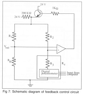
The frequency response of the heaters along with the control circuit was found to be 15 kHz by measuring the time it took for the voltage across a heater to stabilise after a step change in the digital potentiometer position. Because this is much faster than the time scales typically associated with phase change heat transfer processes, the heater temperatures can be considered to be constant.

Calibration

Calibration of the heater array is performed by immersing it in a uniform temperature environment (oven or oil bath) and finding the digital potentiometer wiper position that causes the feedback loop to just begin regulating. The uncertainty in the wiper position is 1 position. Regulation of the heater temperature to within 1 °C can easily be achieved. The heat dissipated by the heater can accurately be measured. Part of this heat is transferred from the heater to the fluid, and part is conducted within the substrate. Since most applications are interested in the former quantity, the heat conducted into the substrate needs to be quantified and subtracted from the total heat dissipation. The uncertainty in wall heat flux therefore depends on how accurately the substrate conduction can be measured, which depends on the application of the heater array. Techniques to determine substrate conduction for two applications are discussed below.

Summary of advantages and disadvantages

The advantage of the microheater array is that it provides time-resolved heat transfer distribution on a surface that has effectively infinite conductivity (constant temperature). Because the temperature is controlled, it allows access to heat transfer regimes that are usually not accessible by constant wall heat flux methods. For example, the microheater array can be used to easily obtain heat transfer data in the transition boiling regime in pool boiling, or in the post CHF regime during spray cooling.

 

Application of Microheater Array to Droplet Cooling

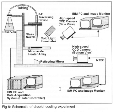
When a droplet strikes a heated surface, it flattens into a thin disk or splat with a thickness which is much smaller than the diameter of the droplet, and high heat fluxes can be obtained due to the formation and evaporation of a thin liquid film on the heated surface. This process is of importance to several industrial applications such as electronic cooling and cooling of steel slabs. A fundamental study of the evaporative heat transfer from a hot surface when a droplet of FC-72 (Tsat=57°C at 1 atm) strikes it was performed (Lee, et al.⁸). A schematic of the setup is shown on Fig 8. Data from the heater array was sampled at 3000 Hz and synchronised with high-speed digital video of the droplet striking the surface. Before the droplet impacted the heater array, the power supplied to each heater is lost only by substrate conduction (the small natural convection from the top and bottom of the substrate was neglected). Because the heater was held at constant temperature, the substrate conduction remained constant even after droplet impact, enabling the heat transferred from the heaters to the liquid to be determined.

 

 

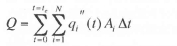
A measure of the accuracy of the heat transfer measurements can be obtained by performing an energy balance on the drop. The total energy transferred from the wall to the drop can be obtained by integrating the measured wall heat transfer over all the heaters and the entire droplet evaporation time:

This energy can be converted into an equivalent droplet diameter (d_eq) using an energy balance on the drop:

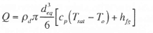
The ratio of the measured initial droplet diameter to d_eq was within 5% for all of the runs, indicating the heat transfer measurements were accurate.

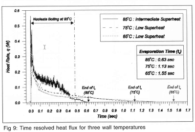
The time variation in wall heat flux over the droplet evaporation time for three wall temperatures is shown in Fig 9. The droplet evaporation time is seen to decrease with increasing wall temperature. The trace for a wall temperature of 85 °C contains a high frequency component from drop impact to about 0.42s. Correlation with the high-speed video indicated that this activity was due to nucleate boiling within splat. Very few bubbles were observed after 0.42s, indicating the end of boiling.

 

 

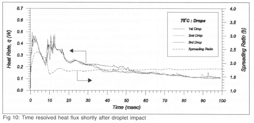
Time resolved heat transfer distributions along with the spreading ratio shortly after impact (0<t<100 ms) for Twall=75°C is shown in Fig 10. The data is seen to be remarkably repeat-able from drop to drop. The oscillations in heat flux are seen to correspond to oscillations in the spread ratio, ß.

 

 

Application of Microheater Array to Boiling Heat Transfer

Boiling is a complex phenomenon where hydrodynamics, heat transfer, mass transfer, and interfacial phenomena are tightly interwoven. It is of importance to processes such as heat exchange, cryogenic fuel storage and transportation, electronic cooling, and material processing due to the large amounts of heat that can be removed with relatively little increase in temperature. An understanding of boiling and critical heat flux is important to the design of heat removal equipment. Although much research in this area has been performed over the past few decades, the mechanisms by which heat is removed from surfaces by boiling are still unclear. Over the past few years, we have used the microheater array to document the pool boiling behavior in earth and microgravity environments. Examples of the heater performance in these environments is given below.

Earth gravity measurements

Saturated boiling on the heater array in the nucleate, CHF, and transition boiling regimes were documented in Rule and Kim⁹. The boiling curve for the heater array facing upward during saturated nucleate boiling for FC-72 at 1 atm is shown on Fig 11. It is seen that obtaining data at critical heat flux and during transition boiling was not a problem since the heaters were operated in constant temperature mode.

 

 

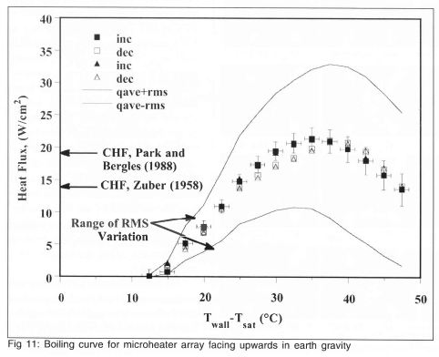
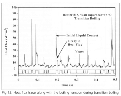
Space-resolved heat transfer measurements indicated that heaters towards the center of the array reached critical heat flux at significantly lower wall superheats (~30°C) than the array averaged heat flux (~35°C) due to the edge heaters blocking the flow of liquid to the inner heaters. It was also possible to distinguish regions on the heater that were covered with vapour, from those where liquid contact occurred in transition boiling by using the time-resolved data from each heater to deduce a boiling function, a bi-modal signal that goes HIGH when boiling occurs on the surface. An example of a time-resolved signal in the transition boiling regime along with the corresponding boiling function is shown on Fig 12. The boiling fraction is defined as the time-average of the boiling function, and represents the time fraction that boiling or enhanced convection occurs on the surface. Within transition boiling, where the surface is alternately wetted by liquid and vapor, the boiling fraction is equivalent to 1 - void fraction, or the liquid fraction. The heat transfer from the edge heaters was observed to be much higher than those for the inner heaters above the temperature corresponding to CHF. The heat transfer during liquid contact in transition boiling, however, was constant for a given wall superheat for the inner heaters, and was observed to decrease with increasing wall superheat.

 

 

Low gravity measurements

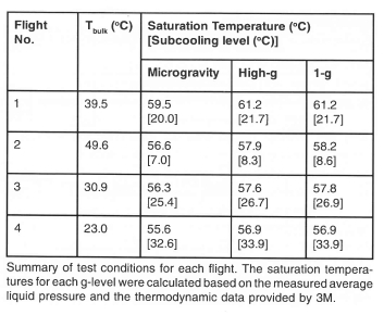
Measurement of boiling in a low gravity environment (0.02 grms) was obtained using NASA's KC-135 aircraft in May 2001. In this series of flights, the bulk liquid temperature was varied from 20°C to 50°C (sub-cooling from 36°C to 6°C), and measurements were made to wall superheats up to 100°C. A summary of the test conditions is given on Table 1. Analysis of this data set is not complete, so the following results should be considered preliminary. Single frames from the high-speed video over the entire range of test conditions obtained through the bottom of the heater are shown on Fig 13. A large primary bubble is seen to form with a size on the order of the heater array. This bubble formed from the coalescence of smaller bubbles that grew on the surface after transition into microgravity.

 

 

 

 

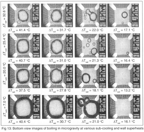
The primary bubble increases in size with increasing bulk fluid temperature and wall superheat, and is fed by smaller satellite bubbles that surround it. For a given bulk temperature, the size of the satellite bubbles decreases with increasing superheat since the size to which they are able to grow is limited by the increasing size of the primary bubble. The motion of the primary bubble at low bulk temperatures was less influenced by g-jitter, since they were smaller and moved about the surface due to coalescence with the satellite bubbles. The size of the primary bubble is determined by a balance between vapour addition, by evaporation of liquid at the bubble base and coalescence with satellite bubbles, and heat loss by condensation through the bubble cap.

Side-view images at selected conditions are shown on Fig 14. Strong Marangoni convection around the bubble was observed to develop, forming a 'jet' of liquid into the bulk liquid. This 'jet' also provided a reaction force on the primary bubble, keeping it on the heater.

 

 

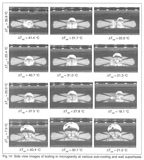
Dryout under the primary bubble occurred for bulk temperatures 39.5 °C and below. Dryout for the edge heaters did not occur, probably due to the flow induced by the Marangoni convection. Dryout over the entire heater array occurred for T_bulk=49.6°C at superheats above 30.7°C - dryout might have occurred as low as 25.7°C, but g-jitter caused the primary bubble to move slightly off the heater array, enabling liquid to rewet the edges of the heater. The contact line of the bubble was stable, and touched the outside of the heater array. Bubble coalescence seemed to be the mechanism by which CHF occurred under the conditions studied.

Boiling curves for microgravity ,earth gravity, and high-g for various sub-coolings are shown on Fig 15. The high-g boiling curve is based on the middle 20 s of the high-g data, and includes data from the pull out (~ 1.6g) and pull up (~ 1.8g). Separate boiling curves were generated from the data taken during the pull out and compared with those during the pull up, but little difference in the curves was observed. The effect of g-jitter must be considered for the microgravity curves. Higher wall superheat is generally associated with larger primary bubbles, which are more sensitive to g-jitter. When the primary bubble moves on the surface or departs due to g-jitter, liquid rewets the surface and results in higher wall heat transfer than would occur in a true microgravity environment. The data at high bulk temperatures and high wall superheats (especially those beyond CHF) may be artificially high as a result.

 

 

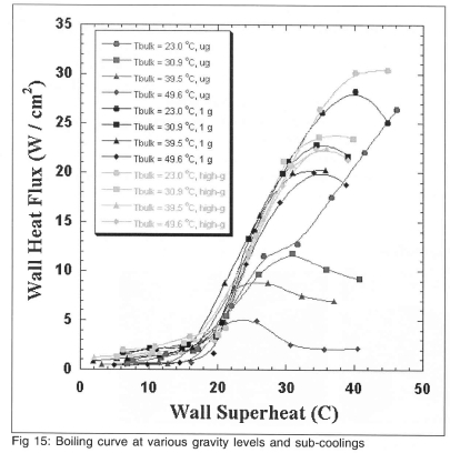
Little effect of sub-cooling is seen in the nucleate boiling regime for the 1 g and high-g data, which is consistent with the observations of previous researchers. The microgravity data tend to follow the 1 g and high-g data for ∆T_sat<20°C, but drop below them for higher superheats as the primary bubble causes dryout over a successively larger fraction of the heater. CHF for the microgravity curves are significantly lower than those for the 1 g and high-g data.

The time averaged heat flux distribution from each heater in the array is shown on Fig 16. The scale has been kept the same for all images to highlight the change in heat transfer with wall superheat and sub-cooling.

 

 

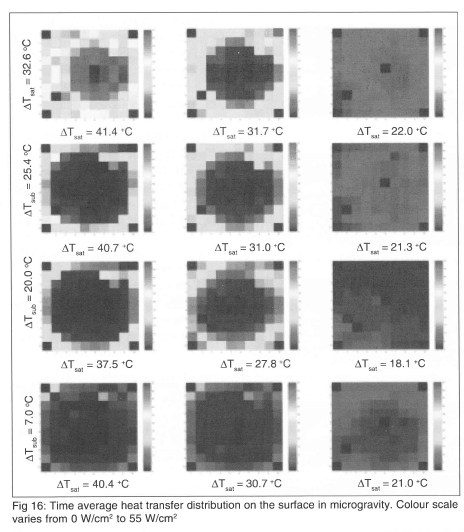
Very little heat transfer is associated with the primary bubble, even along the contact line. Much higher heat transfer rates are associated with the rapid growth and coalescence process of the satellite bubbles. A significant amount of the surface dries out before CHF. CHF occurs when the dry spot size grows faster than the increase in heat transfer outside the primary bubble.

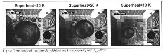
The time resolved heat flux distribution for T_bulk=20.0°C at three superheats are shown in Fig 17. As was noted for Fig 16, much higher heat transfer is associated with the small scale boiling on the array. In order to conditionally sample the heat flux only when boiling occurs on the surface, a boiling function was generated from the time-resolved heat flux data. This function is a bimodal signal that is set to HIGH when boiling occurs on the surface, and LOW otherwise. Details of how the boiling function is generated are discussed in Rule and Kim⁹. The time averaged heat flux obtained by sampling the data only when the boiling function is HIGH is referred to as the nucleate boiling heat flux, and is a measure of the heat transfer associated with the satellite bubbles.

 

 

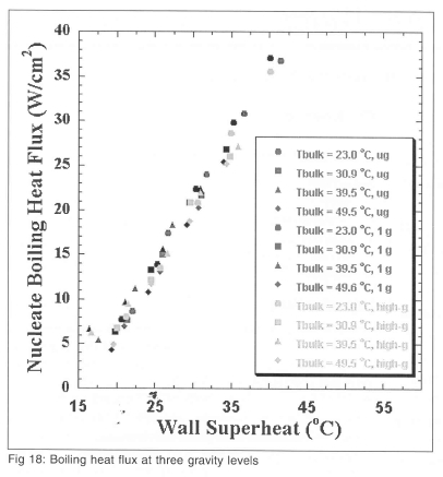
Boiling curves generated from the nucleate boiling heat flux for microgravity, earth gravity, and high-g environments are compared on Fig 18. It is seen that the nucleate boiling heat flux collapses onto a single curve, indicating that the small scale boiling is independent of sub-cooling and gravity level. This suggests that if one is able to predict the extent of the dry area in microgravity, then one could predict the microgravity boiling curve from earth or high gravity boiling heat flux data.

 

 

Other Potential Applications

The microheater array can be used for a wide range of other applications as well. Consider the case where the heaters are constructed to form a linear array, and operated in the same way described above. This linear array can then be capped off, forming a micro-channel. The heat transfer coefficient distribution within this micro-channel can then be measured, providing information about the flow regimes and heat transfer mechanisms. Visualisation studies can also be conducted since the microheater array is semi-transparent.

The linear array can also be operated as a bubble pump. Bubbles can be nucleated at intervals along the heater array. If the bubbles are then shifted along the array by successively heating adjacent heaters, the liquid between the bubbles can be pumped through the channel. The advantages to such a pump are numerous. Firstly, it has no moving parts to wear out. Secondly, because it takes a relatively high force to dislodge a bubble from a heater, high pressure differentials can be created across the channel. Third, because the bubble can be shifted along the channel at high velocities, high flow rates can be achieved.

The heater array can be used during combustion catalysis experiments to measure the rate of reactions. Consider the case where the platinum heaters are held at uniform temperature. With no reaction on the surface, a certain amount of power is required to keep the heater at a uniform temperature due to substrate conduction losses. Exothermic reactions on the surface of the platinum will cause the power required to keep the heater at a constant temperature to decrease, enabling the heat released by the reaction to be measured.

 

Conclusions

The use of two techniques to determine space and time-resolved heat transfer distributions on a wall has been described. Demonstration of the constant temperature heater array has been performed for phase change processes involving boiling and droplet cooling. This technology is expected to be applicable to a wide range of additional phenomena.

 

Acknowledgments

This work received support from the Office of Biological and Physical Science at NASA Headquarters, the Laboratory for Physical Science, and the Air Force Research Laboratory. Their support is gratefully acknowledged.

 

References

1. Bayazit, BB, Hollingsworth, DK, and Witte, LC, "Heat transfer enhancement caused by sliding bubbles", Proceedings of the 2001 National Heat Transfer Conference, Anaheim, CA.

2. Kenning, DBR, Bustnes, OE, and Yan, Y (2000) "Heat transfer to a sliding vapor bubble", Proceedings of the Engineering Foundation Conference on Boiling Phenomena and Emerging Applications, Anchorage, AK.

3. Theofanous, TG, Tu, JP, Dinh, TN, Salmassi, T, Dinh, AT and Gasljevic, K," Physics of boiling at burnout." Fifth Microgravity Fluid Physics and Transport Phenomena, Cleveland, OH, August 9-11, 2000.

4. Fath, HS, and Judd, RL, 1978, "Influence of System Pressure on Microlayer Evaporation Heat Transfer," ASME Journal of Heat Transfer, Vol. 100, pp. 49-55.         [ Links ]

5. Koffman and Plesset (1983) "Experimental Observations of the Microlayer in Vapor Bubble Growth on a Heated Surface", Journal of Heat Transfer, Vol. 105, pp. 625-632.         [ Links ]

6. Sheats, JR, Antoniadis, H, Hueschen, M, Leonard, W, Miller, J, Moon, R, Roitman, D, and Stocking, A, "Organic Electroluminescent Devices." Science 1996, 273,884-888.         [ Links ]

7. Incropera, FP and Dewitt, DP, 1996, Fundamentals of Heat and Mass Transfer, Fourth Edition, John Wiley and Sons.

8. Lee J, Kim, J, and Kiger, KT, (2000)" Time and Space Resolved Heat Transfer Characteristics of Single Droplet Cooling Using Microscale Heater Arrays", International Journal of Heat and Fluid Flow, Vol. 22, pp. 188-200.         [ Links ]

9. Rule, T and Kim, J, (1999) "Heat Transfer Behavior on Small Horizontal Heaters During Pool Boiling of FC-72", Journal of Heat Transfer, Vol. 121, No. 2, pp. 386-393.         [ Links ]