PROFESSIONAL TECHNICAL AND SCIENTIFIC PAPERS

 

Testing sample representivity using particle size distribution

 

 

R.C.A. Minnitt^I; P. Minkkinen^II

^ISchool of Mining Engineering, University of the Witwatersrand, Johannesburg, South Africa. http://orcid.org/0000-0002-0267-8152
^IILappeenranta University of Technology, Finland

Correspondence

 

 

---

ABSTRACT

Particle size distribution analysis is important to many industries for assessing product quality, process efficiency, and compliance with contractual standards, while ensuring sample accuracy, and representativeness. Inaccurate particle size distribution results, arising from fines due to excessive handling can lead to penalties and buyer-seller disputes. A non-representative particle size distribution means samples will not accurately represent the chemical components either. Sampling blasthole cuttings poses challenges due to large material volumes, segregation, and uneven settling of particles in dense gold bearing ores. Commonly used sampling methods, such as spear or sectoral sampling, may lack representativeness. Particle size distribution analysis is crucial for evaluating sampling methods by comparing test sample representativeness against a reference standard derived from multiple particle size distribution analyses. Acceptable samples must fall within the 97.5% confidence intervals of the standard; deviations analyses lying outside these boundaries indicate a strong likelihood of segregation errors. A case study demonstrates this approach by using a 6.005 kg benchmark sample to assess two additional samples (1 kg and 5 kg), highlighting particle size distribution's role in detecting sampling errors and refining protocols. An example of three test samples collected from reverse circulation drill cuttings compared to a standard reference sample is presented to illustrate a quality assurance/quality control procedure for reverse circulation drilling.

Keywords: particle size distribution, mass fraction, sample representivity, relative difference, reverse circulation drilling

---

 

 

Importance of particle size distribution in sampling

Analysis of particle size distribution (PSD) is essential in industries for evaluating product quality, assessing process efficiency, ensuring compliance with contractual terms, validating sampling system accuracy, and confirming sample representativeness (Pitard, 2019). Accurate PSD results are critical for decision-making in industries reliant on granular material processing. Contracts may impose penalties on specific granulometric classes that could disrupt process operations. For instance, penalties for fines necessitate avoiding breakage during sample extraction, as this can artificially produce fines and introduce a positive bias in PSD analysis. Excessive handling operations, such as loading, unloading, and sampling, further exacerbate biases in commodities like coal, coke, iron ore, manganese ore, bauxite, and alumina, creating conflicting perspectives between sellers and buyers regarding material quality.

Ensuring a representative sample of the size distribution in a lot is paramount. According to Pitard (2019), if a sample is not representative of the size distribution, it cannot accurately represent any other characteristic. A fundamental rule is that "a sample mass that is too small to justly represent all size fractions cannot provide a sample representative of anything else" (Pitard, 1993; 2019). Segregation, inherent in lots with significant size variation, must be minimised through unbiased sampling methods that yield replicate samples closely aligned with the standard PSD. Proper sampling processes are essential to mitigate segregation and delimitation errors, especially in a case such as sampling blasthole cuttings.

Sampling blasthole cuttings involves unique challenges due to the high mass of material, which can reach several tonnes, and the effects of segregation and delimitation errors. In vein-type ores with high density mineralisation, such as gold and base metal sulphides, these challenges are pronounced as cuttings settle unevenly around the drill string. Sampling methods like spear or sectoral sampling, although commonly used, often fail to ensure representativeness. Accurate sampling requires attention to the depth and uniformity of material collection, particularly in the first few metres of drilling, where cuttings are minimal and often contaminated with sub-drill material.

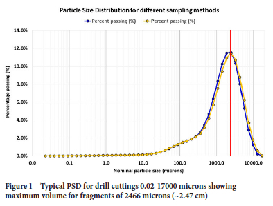
A typical procedure for sampling drill cuttings involves laying a tarpaulin around the hole to prevent ground contamination and using triangular sectoral trays to collect samples continuously over a 3-metre drill depth. For a 200 mm drill hole, this depth produces approximately 270-300 kg of cuttings, from which 35-40 kg is collected and split into two 5 kg samples for PSD and chemical analysis. These samples are compared to ensure consistency and representativeness. A typical PSD for two samples of drill cuttings 0.02-17000 microns showing maximum volume for fragments of 2466 microns (2.47 cm) is shown in Figure 1.

 

 

Accurate representation of particle size distribution in sampling

An accurate particle size distribution (PSD) measurement ensures that the sample truly reflects the bulk material's size characteristics-critical because if PSD does not accurately represent the size distribution, it cannot accurately represent anything else. In pharmaceuticals, incorrect PSD alters drug performance; in mining, it reduces recovery rates. However, achieving accuracy is challenging due to grouping and segregation, where particles separate by size during handling.

Proper sampling techniques are essential to minimise bias. Incremental sampling collects material from multiple locations, while coning and quartering homogenises samples. Analytical methods must match material properties: Laser diffraction suits high-throughput analysis, dynamic image analysis captures particle shape, and sieving remains reliable for coarse fractions. Statistical validation, including confidence intervals and percentile metrics (D10/D50/D90), confirms whether results align with reference standards.

The financial liabilities and compromised operational efficiency arise due to non-representative sampling, and inaccurate PSD analysis. For example, contractual penalties may be imposed if product specifications (e.g., fines content <10%) are violated due to biased sampling. In iron ore trading, a 1% deviation from contracted PSD can trigger penalties exceeding USD1 million per shipment (Pitard, 2019). Under-sampling of coarse gold bearing particles because of incorrect PSD data leads to suboptimal grinding or inadequate liberation, reducing recovery rates by 5%-15% (Minkkinen et al., 2015). In 2018, losses of USD2.5 million, attributed to misrepresentation of PSD from spear sampling, led to costly arbitration regarding bauxite shipment quality (Pitard, 2019). Non-compliance with airborne coal dust standards may incur fines if PSD underestimates fines generation.

PSD analysis is instrumental in evaluating sampling methods. For instance, the representativeness of spear and sectoral sampling can be tested against a reference standard compiled from PSD analyses of ten or more samples collected from multiple cones around geologically similar blast holes. Upper and lower 97.5% confidence intervals (CIs) for the reference standard establish a framework for comparison. A sample's mass fractions must fall within these CIs to be deemed acceptable. Significant deviations indicate that segregation errors affect the representativeness of the sampling method (Pitard, 1993; 2019). Reliable PSD demands unbiased sampling, appropriate instrumentation, and statistical rigor. By adhering to best practices, industries can avoid financial losses, ensure compliance, and maintain quality control, underscoring PSD's vital role in material science and industrial applications.

A case study by Minkkinen et al. (2015) highlights the application of PSD analysis in assessing sampling methods. A 6005 g standard sample taken with a new device served as the benchmark. Two additional samples, weighing 1 kg and 5 kg, respectively, were compared to the standard. This comparative analysis demonstrated the utility of PSD in identifying sampling errors and improving sampling protocols.

 

Derivation of constitutional heterogeneity and related equations

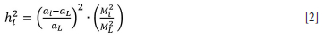
A variety of methods exists by which the relative sampling variance may be derived, including the approach provided by Gy (2004), which reflects real-world complexity. This derivation quantifies the heterogeneity contribution (hi) of every fragment i in the lot to the variance based on the deviation of grades (α_i-α_L), and the mass ratio (M_i/(M_i), as shown in Equation 1:

While the mean of all h_i is zero, the variance is:

The dimensionless number h_i with a mean of zero, was central to Gy's (2004) first "equiprobable" model for the sampling variance as early as 1950, and led to the definition of the constitutional heterogeneity CHl of the lot, defined as the variance of h_i in the population of N_f fragments comprising the lot:

This parameter can only be rarely estimated so it is replaced by using the idea of fragment heterogeneity via the heterogeneity invariant (HI_l) or intrinsic heterogeneity (IH_l), which is far easier to define (Gy, 2004; Pitard, 2019). This accounts for the intrinsic fragment variability and quantifies the relative sampling variance, which sums the squared deviations of individual fragment grades (a_i) and masses (M_i) from the lot average:

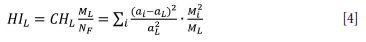
Where a_L and M_L are the grade of the lot and the mass of the lot, respectively. This approach addresses non-uniform, real-world ores, for complex lots affected by clustering and variable liberation and which leads to Gy's formula, σ_R² (α_s) ≈

In many industries, analysing the particle size distribution of a material is a critical factor because it helps evaluate product quality, measure process effectiveness, ensure compliance with contractual agreements, verify sampling system precision, and confirm that collected samples accurately represent the material (Pitard, 2019). Pierre Gy (1992; 1998) derived an equation, which can be used to estimate the relative variance of the fundamental sampling error (FSE) from the mass fractions of each size fraction, as determined by PSD analysis. The heterogeneity invariant (ΉI) represents the relative variance of the FSE for a unit mass sample, typically 1 gram. A full derivation of the formula for HI_l provided by Pitard (2019), is not repeated here, but his formula is shown in Equation 5:

Minkkinen et al. (2015) modified this formula, as shown in Equation 6, to provide an acceptable estimate of HI by a standard sieve analysis for each size class i.

where

i = the size class

a_i = mass fraction of size class i

v_i = average particle size in class I (this should be d_i) is estimated from the sieve openings; f is the particle shape factor (default is 0.5 for irregular particles)

p_i = density of particles in size class i.

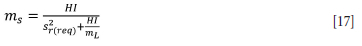
Given HIi, s²fse can be estimated for different sample sizes to be sieved from the test material using Equation 7:

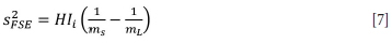
where

m_s = sample mass to be sieved

m_L = mass of the lot from which the sample is taken.

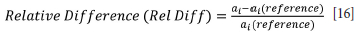
If the sampling method is unbiased and effectively minimises segregation effects, the FSE error variance (s²fse) of replicate samples should be close to that obtained for the standard by using the above equations. It is also possible to calculate a confidence interval for a given size distribution; the relative difference for each mass fraction (a_i) for each size fraction of the test sample should lie within the confidence limits of a standard sample. If the PSD sample is supported by determination of silicate or elemental composition, the correlation between size classes can be investigated using principal components analysis (PCA). These methods provide a way of determining if a given sampling method or technology is extracting a correct, and therefore representative sample. Where it can be shown that the samples taken are representative of the original lot, and the method can be applied in practice and confidence intervals can be calculated for a given size distribution.

The average volume of fragments between two screens is given by Equation 8:

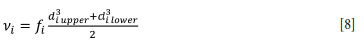
where f_i is the shape factor; a default value of 0.52 should be used; the average fragment mass per class interval is the product of the density and V_i.

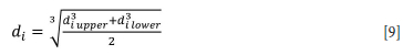
The nominal fragment size is calculated slightly differently using Equation 9.

It is important to note how heterogeneity invariant (HIi), the constitution heterogeneity (CH_i), and the variance of the FSE (s²fse) are related, as shown in Equations 1, 2 and 3; when m_s is much less than m_L:

If the sample forms a significant part of the lot from which it is taken, then a correction must be made in estimating the sample variance.

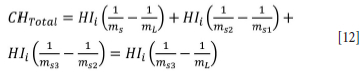
If the primary sample m_s1 is taken from a lot of size m_L, and sample m_s2 is taken from the primary sample, and sample m_s3 is taken from the secondary sample and then sieved, the variance of this three-step process, if the size distribution is not changed, is:

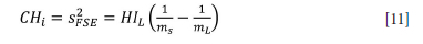
The constitution heterogeneity (CHi) is the relative variance of the sampling error, scaled by sample and lot sizes, and the relative standard deviation (s_ri) converts CH_i to standard deviation for size classes, S_r as follows:

If the relative standard deviation is given in percentages, sri should be multiplied by 100. The fundamental sampling variance s²FSE gives the variance of an ideal sampling process, i.e., the material of the lot is a random mixture of its constituents, and the sampling process is correct. If there is segregation in the lot or sampling devices are not correctly designed or operated, experimental variances will be larger than those calculated from the equation for HI_i and relative difference of a_i will be evident.

Practical applications allow the uncertainty in the results to be estimated using the absolute standard deviation to calculate and plot confidence intervals for different size fractions. Approximate confidence intervals CI for the size fractions is shown in Equation 14.

Where a_i is the mass fraction, k is the coverage factor of 1.96, giving 95% and 3.0, giving 97.5% confidence intervals and s_r is the standard deviation.

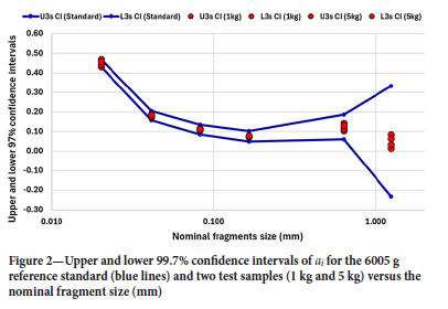
The confidence intervals for mass fractions are derived from the relative standard deviation (s_r), which is itself a function of the constitution heterogeneity (CH) and heterogeneity invariant (HI). Beginning with Equation 1, CH is defined as the scaled sampling error variance (Equation 6). For a 97.5% CI, the interval width is k X s_r, where k = 1.96 (or 3.0 for 99.7% CI, Figure 2). Here, s_r = CH_i (Equation 13), directly linking HI (Equation 5) to the practical uncertainty bounds. This chain of dependencies ensures that the CIs reflect both the intrinsic heterogeneity (HI) and sampling process (CH).

 

 

Multivariate analysis via principal components analysis (PCA)

Where PSD data are supplemented by compositional assays (e.g., SiO₂ or Au content), principal components analysis (PCA) can identify correlations between size classes and chemical heterogeneity. For example, in gold ores, PCA might reveal that +2 cm fragments correlate with nuggety gold, while fines dominate silicate-rich fractions. Such analysis helps validate whether PSD representativeness extends to compositional representativeness. A case study by Pitard (2019) demonstrated that PCA of paired PSD and assay data reduced sampling bias by 30% in iron ore processing.

 

Testing sample efficiency with particle size distribution

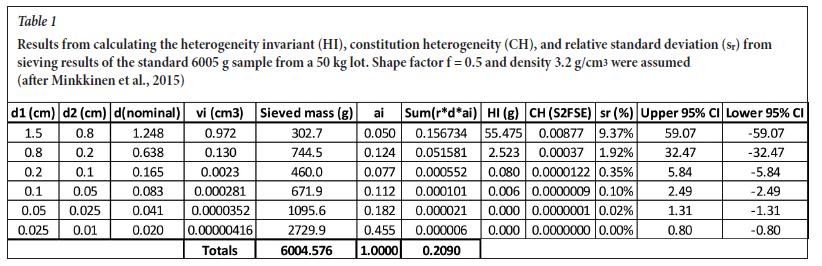
The efficiency of two different sampling methods was tested by Minkkinen et al. (2015), the results of which are shown in Table 1.

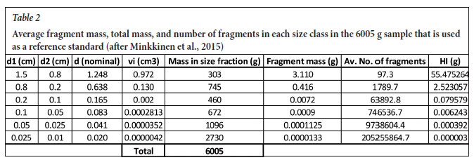
Table 1 provides a linear sequence of calculations, including the nominal fragment size, the mass fraction (a_i), the heterogeneity invariant (HI, Equation 5), and the fundamental sampling error (CH, Equation 11), the standard deviation (sr %, Equation 9), and the lower and upper confidence limit calculations for the reference standard. The average fragment mass per size fraction (vi*density), total mass of fragments, and the average number of fragments in each of the six size classes sieved from the 6005 g standard sample are shown in Table 2.

The sampling variance of a particle mixture is a function of the number of the analyte particles in the sample. When the particle size is reduced, the number of fragments rapidly increases and, as a result, HI decreases (Table 2). If a reliable result for the coarsest fraction in the sample is necessary, then the number of the analyte particles determines the minimum sample size that should be used.

 

Confidence intervals and their significance in mass fraction analysis

A confidence interval (CI) is a range of values, derived from a dataset, that is likely to contain the true value of the mean with a specified level of confidence and provides a measure of uncertainty associated with a sample estimate. The 95% confidence interval used here means that for multiple repetition of sample analyses, 95% of the calculated means would contain the true value. In the context of PSD, which measures the proportion of a specific size fraction in a sample, confidence intervals are used to estimate precision by determining how accurately the measured mass fraction represents the true value in the standard sample. Confidence limits provide a framework in which reliability and repeatability of sampling methods can be determined and provide a visual means of identifying statistically significant differences between sampling methods.

In quality assurance and quality control (QA/QC), confidence intervals can highlight whether the variation in measured mass fractions is within acceptable limits. CIs provide a quantitative way to quantify the uncertainty in mass fraction estimates. Narrow intervals indicate high precision, while wide intervals suggest greater uncertainty. Confidence intervals support informed decisions about material quality, compliance with specifications, and production adjustments. Where relative differences between mass fractions lie within the limits for the standard, there is no significant difference between sampling methods, whereas points lying outside the limits indicate a statistically significant difference. Wider confidence intervals often result from small sample sizes (Table 1) and this insight can guide the requirements of minimum sample mass and the design of sampling protocols to improve accuracy. CIs can reveal systematic biases in measurements, especially when comparing duplicate samples or different sampling methods. In summary, confidence intervals are critical in mass fraction analysis for understanding the precision, reliability, and statistical significance of analytical results of different sampling methods.

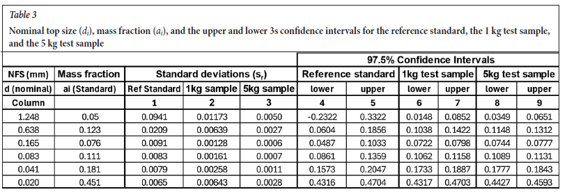
The 99.75% upper and lower confidence limits for the mass fraction (a_i) in Table 3 for the 1 kg and 5 kg samples are calculated using Equation 15:

Table 3 shows the confidence intervals for the mass fractions (a_i) in each size fraction for the reference standard as well as for 1 kg and 5 kg tests samples, calculated using the experimental HI values (Equation 1). Confidence intervals of the 1 kg and 5 kg samples can now be placed in the framework for the standard sample, as shown in Figure 2.

The 3 upper and 3 lower confidence intervals for the reference standard (Table 3, columns 4 and 5), calculated using Equation 12 are plotted against the nominal fragments size (mm) as shown in Figure 2 and form an important starting point for the Minkkinen et al. (2015) analysis.

The upper and lower confidence intervals for the 1 kg and 5 kg test samples are plotted as points which all lie between the CIs of the reference standard, indicating that they are acceptable and thus representative of the PSD derived by the test methods.

The calculated confidence intervals for the replicate samples lie well within the limits for the standard sample, indicating that despite the significant size distribution between the samples and the reference standard, the sampling method tested for sample masses of different sizes is correct and unbiased, and therefore able to minimise segregation.

 

Minimum sample size for a given precision requirement

The minimum sample size for precision to achieve a desired relative standard deviation s_r (for an ideal mixture and sampling system) is given by Equation 17.

The calculations assume ideal conditions. Factors like segregation, incorrect sampling equipment, and approximation of particle properties can introduce errors. Results outside confidence intervals suggest sampling or material issues. If fewer than 16 fragments from the coarsest fraction are included, symmetric confidence intervals are invalid. To account for uncertainties, double the theoretical minimum sample size and reducing sample size requires combining multiple increments to minimise errors.

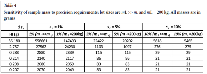
By applying these principles, one can evaluate and improve the reliability of sampling processes for size distribution and compositional analyses. Table 4 shows the sieve results obtained from one of the experimental drill holes.

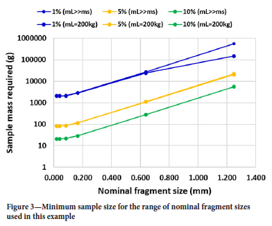
Table 4 shows how the theoretical minimum sample size depends on the required uncertainty of sampling given as the relative standard deviation: 1%, 5%, and 10%. It quantifies the precision-cost trade-off by demonstrating how the minimum sample mass (m_s) scales nonlinearly with the desired precision (sr(req)). For instance, reducing s_r from 10% to 1% requires a 100-fold increase in m_s (Equation 13). This sensitivity is critical for cost-benefit decisions. Sample sizes were calculated for two different lot sizes: 200 kg (sample taken from a pile) and from a lot much larger, about 20 t, than the sample (primary sample taken from a large target). Where high precision is required, as in compliance testing, a 147 kg sample is required for 1% Sr in the coarsest fraction (Table 4). For less demanding precision such as exploration sampling a 10% Sr may suffice, allowing smaller samples (1.47 kg). The exponential relationship (Figure 3) underscores the trade-off between precision and operational feasibility. The changes in sample mass for a change in nominal fragment size are shown in Figure 3.

 

 

Example for a complete particle size distribution

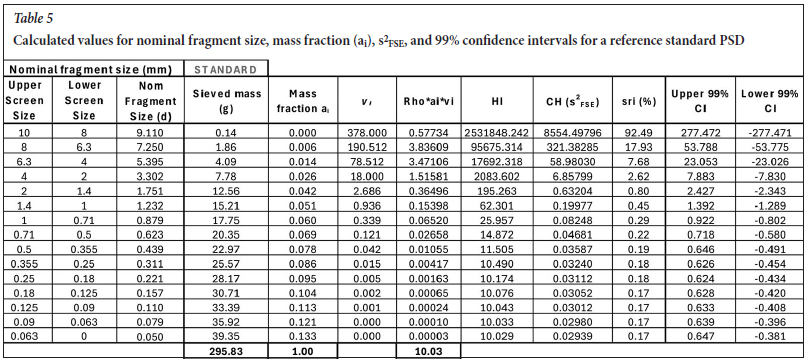
A set of PSD data was obtained as a standard bulk composite sample from cuttings in a cone around a blast hole, as shown in Table 5. The performance of another three samples SAMPLE 1, SAMPLE 2, and SAMPLE 3, collected in adjacent blast holes was compared against this standard.

The data in Table 5, columns 1, 2, and 4, the two screen sizes, and the sieved mass (g) are typical results for a reference standard PSD analysis. The primary data are the upper and lower screen sizes used (columns 1 and 2), and the sieved mass is that retained on top of each screen. The nominal top size (column 3) for each

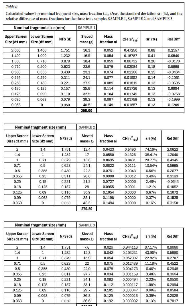
size fraction is calculated using Equation 9, and the volume of each size fraction v_i (column 6) is calculated using Equation 8. The mass fraction, a_i is the proportion of the mass of the size fraction relative to the total sieved mass (295.83 g). The sum of the product density, nominal size, and mass fraction for each mass fraction is calculated (10.03 g), a value that is substituted into Equation 1 to give the HI for each size fraction, and from which the constitution heterogeneity (CH), and the relative variance of the sampling error (s²fse) is calculated, using Equation 11. The relative standard deviation s_r (%) is then calculated using Equation 9 and the upper 99.7% and lower 99.7% confidence intervals (columns 11 and 12) can be calculated, and are plotted as the upper and lower 99.7% confidence intervals forming the framework against which any samples can be tested. The data for the three test samples, SAMPLE 1, SAMPLE 2, and SAMPLE 3, are listed in Table 6.

The relative difference between the mass fractions of the reference standard (Table 5) and the three test samples, is calculated using Equation 16 and is shown for SAMPLE 1, SAMPLE 2, and SAMPLE 3, in column 8 of Table 6. These values are plotted against the confidence intervals of the standard, as shown in Figure 4.

 

 

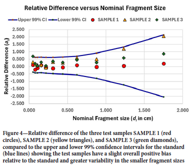
Comparison of the mass fraction at different size fractions of the sample against the 3 times confidence intervals for the standard indicates that these lie well within the limits of the standard and suggests that the PSD of the test samples is acceptable, with the conclusion that the three test samples of blast hole cuttings may be considered representative of the lot. It should be noted that the Cls widen considerably for size fractions over 1.75 cm (Table 6, columns 11 and 12 for size fractions > 1.75 cm), so data from this section of the analyses have not been plotted in Figure 4.

 

Best practices for field sampling

To ensure representative PSD analysis while minimising financial and operational risks, the field sampling protocol should minimise excessive handling and transfers to avoid generating fines and a biased PSD. The use of conveyor belt samplers or automated dividers (e.g., rotary splitters) instead of spears or grab sampling is recommended (Minnitt, 2024; Trottier, Dhodapkar, 2012). For blasthole cuttings, one should collect increments directly from the drill stream to avoid segregation (Dominy et al., 2018). In terms of the number of increments and the sample mass, Gy (1992) recommends >30 increments per lot to mitigate segregation and grouping errors, while for highly heterogeneous gold ores it is recommended to use Equation 13 to calculate minimum sample mass (see Table 4). The use of crushers and splitters should be calibrated and validated for consistency using certified reference materials, while field samples should be compared against a cone-quartered bulk standard to detect segregation. Paired PSD and assay checks using PCA for size and chemical correlations should be used to validate representativeness, monitor confidence intervals (Figure 2), and flag outliers (>97.5% CI) for re-sampling.

 

Conclusions

Confidence intervals (Cls) are essential for evaluating the precision and reliability of PSD analyses in sampling methods. Upper and lower 99% Cls mean that repeated analyses would capture the true mean 99% of the time and provide the framework to compare test samples against a reference standard. The PSD-derived Cls indicate whether mass fractions of test samples fall within acceptable limits, identifying potential segregation errors.

The study by Minkkinen et al. (2015) applies PSD analysis to assess sampling methods, using a 6005 g standard sample as a benchmark. Two test samples of 1 kg and 5 kg were compared within the standard framework, and their confidence intervals fell within the reference standard's limits, confirming their representativeness.

A minimum sample size calculation ensures precision, with larger samples required for lower uncertainty. Systematic biases and variability in test samples can be identified by comparing their relative differences against the reference standard's Cls. The final analysis of blast hole cuttings showed that the test samples were within acceptable limits, except for larger size fractions (>1.75 cm), where the widening of the Cls reduces the reliability. These findings highlight the importance of PSD-based Cls in ensuring sample representivity for blast hole and RC drill cuttings, to improve sampling protocols where necessary and ensure reliable material characterisation.

 

Acknowledgements

The authors express their gratitude to Maunu Mänttäri of RTD Department Sandvik Mining and Rock Technology Oy, Tampere, Finland for his kind permission to use the PSD data presented in Samples 1, 2, and 3.

 

References

Dominy, S.C., Glass, H.J., O'Connor, L., Lam, C.K., Purevgerel, S., Minnitt, RCA. 2018. lntegrating the Theory of Sampling into Underground Mine Grade Control Strategies. Minerals, vol. 8, no. 6, p. 232. https://doi.org/10.3390/min8060232        [ Links ]

Gy, P. M. 1992. Sampling of Heterogeneous and Dynamic Material Systems. Elsevier, Amsterdam.         [ Links ]

Gy, P.M. 1998. Sampling for Analytical Purposes. John Wiley & Sons Ltd, Chichester.         [ Links ]

Minkkinen, P., Auranen, l., Ruotsalainen, L., Auranen, J. 2015. Comparison of sampling methods by using size distribution analysis. Proceedings of the World Conference on Sampling and Blending 2015, WCSB7. TOS forum lssue 5, 2015. www.impublications.com/wcsb7. doi: 10.1255/tosf.63. 175-185        [ Links ]

Minnitt, R.C.A. 2024. Mid-Boyd crusher and sample divider test results. Scott | Mid-Boyd Crusher and Sample Divider Test Results        [ Links ]

Pitard, F. F. 2019. Theory of Sampling and Sampling Practice. Third Edition. Boca Raton: Taylor & Francis, 2019. 693 p.         [ Links ]

Pitard, F. F. 1993. Pierre Gy's sampling theory and sampling practice: Heterogeneity, sampling correctness, and statistical process control. Second Edition. CRC Press, Taylor & Francis Group, 2nd ed. c1993. 488p.         [ Links ]

Trottier, R., Dhodapkar, S. 2012. Sampling Particulate Materials the Right Way April 1, 2012, The Dow Chemical Company. Sampling Particulate Materials the Right Way - Chemical Engineering | Page 1        [ Links ]

 

 

Correspondence:
R.C.A. Minnitt
Email: Richard.Minnitt@wits.ac.za

Received: 10 Feb. 2025
Revised: 21 Jul. 2025
Accepted: 25 Aug. 2025
Published: September 2025