RESEARCH ARTICLE

 

Machine-learning forecasting model of tuberculosis cases among children in South Africa

 

 

Adeboye Azeez^{I, II}; Georgeleen Osuji^I; Ruffin Mutambayi^I; James Ndege^I

^IDepartment of Computational Sciences, University of Fort Hare, Alice, South Africa
^IIGastrointestinal Research Unit (GIT), Department of Surgery, Faculty of Health Sciences, University of the Free State, Bloemfontein, South Africa

Correspondence

 

 

---

ABSTRACT

Globally, children and young adolescents under 15 years old constitute approximately 11% of all tuberculosis (TB) cases, with a growing concern over TB infections in children under 5 years old, especially in resource-limited settings. Nonetheless, the true extent of TB burden among children remains inadequately explored in South Africa. The application of a random forest-Bayesian autoregressive integrated moving average (RF-BARIMA) model for infectious disease prediction has not been previously employed to study TB in children. In this study, we employed the RF-BARIMA model to forecast TB incidences, from 2010 to 2019, among children under 5 years old in South Africa's Eastern Cape Province. Comparative analysis demonstrated that the RF-BARIMA model outperformed other models in predictive accuracy and forecast capability. Qur predictions revealed a projected mean of 0.4122 TB cases per month in 2022, with an effective sample size of 4054 TB cases in the Eastern Cape Province. These findings indicate a prospective reduction of 1670.85 TB cases among children under 5 years old in the coming years. The RF-BARIMA model offers enhanced predictive and forecast accuracy in comparison to the single Bayesian ARIMA model. These results provide compelling evidence of significant under-reporting and potentially elevated TB incidence among children under 5 years old in South Africa's Eastern Cape Province, raising important implications for public health policy and intervention strategies.
SIGNIFICANCE:
Childhood tuberculosis (TB) in South Africa is a significant concern, with the majority of cases occurring in children aged 0-4 years. The burden in children mirrors the high burden of the adult epidemic in the country. The RF-BARIMA model integrates the non-linear pattern of random forest with the probabilistic time series forecasting strengths of Bayesian ARIMA, aiming to improve prediction accuracy and quantify uncertainty in the forecasts. The results lead to a call for urgent public health policy and intervention strategies to address the under-reporting and elevated TB incidence in this vulnerable demographic, further reinforcing the study's global significance.

Keywords: ARIMA model, Bayesian, random forest, machine learning, tuberculosis

---

 

 

Introduction

In recent years, despite increased global awareness of the prevalence of paediatric tuberculosis (TB), the development of machine-learning algorithms to enhance diagnostic methods has been limited. In 2021, approximately 1.2 million children were estimated to contract TB, but only a third of children aged 0 to 5 years received proper care and were reported in national TB programmes.^1,2 Although collecting and testing many samples may increase diagnostic yield and improve diagnosis, implementation at the primary care level, where the need for adequate diagnostic tools is most significant, remains challenging.^3,4 Machine-learning algorithms are computational methods that enable systems to learn from data and make predictions or decisions without explicit programming. Popular machine-learning models for TB incidence prediction - such as autoregressive integrated moving average (ARIMA), seasonal ARIMA, decision trees and neural networks like recurrent (RNN) and backpropagation (BPNN) neural networks - have shown high accuracy rates in diagnosing TB from clinical data.^5,6 Machine-learning algorithms can be used to predict incidence rates, improve diagnostics and close the treatment gap in childhood TB.^7,8 Machine learning has become a valuable tool for forecasting TB cases among children, particularly in resource-limited settings. Models such as ARIMA, hybrid ARIMA and artificial neural networks (ANN), and deep learning approaches have been employed to improve predictive accuracy and support targeted public health interventions. Hybrid models, especially ARIMA-ANN, have outperformed traditional ARIMa methods, showing significantly better performance (p < 0.001).⁹ Deep learning models like convolutional neural network combined with long short-term memory (CNN-LSTM) and multilayer perceptron (MLP) have also demonstrated strong predictive capability, achieving minimal forecasting errors.¹⁰

The World Health Organization (WHQ) has conditionally approved a new TB diagnostic algorithm with a sensitivity of 85% when using chest X-ray features (visible signs of tB conditions), or 30% specificity without them.¹¹ However, the algorithm still requires further validation and training for accurate interpretation. Various forecasting models are employed for infectious diseases, including grey prediction^12,13, exponential smoothing prediction¹⁴, dynamic model¹⁵, Box-Jenkins^16,17, and others. When using the forecasting method to attain accurate prediction, models are developed based on the features of the time series, such as historical incidence rates, seasonality patterns, demographic data, public health interventions, social and environmental factors, and population mobility. When the prediction effect of a single model is not optimal, many studies choose the combination model prediction approach.^18-21 The combined model can absorb the advantages of two or more methods in order to achieve greater forecast accuracy.

Bayesian inference is a widely used method for analysing conditional probabilities of events, such as predicting hierarchy time series data²², seasonality^23,24, and multi-step-ahead prediction²⁵. It is also applied in general estimation, prediction tasks²⁶ and statistical analysis²⁷. In time-series forecasting, the Bayesian method can be employed to forecast using a Kalman filter and smoothing technique and the Markov chain Monte Carlo (MCMC) method.²⁸ Qne study demonstrated the effectiveness of Bayesian networks in accurately predicting clinical parameters of chronic obstructive pulmonary disease (CQPD) patients' time series data.²⁹ This not only improved computational efficiency but also optimised the modelling process. Additionally, dynamic Bayesian networks, which combine Kalman filtering models and echoing neural networks, have been utilised to predict multi-step-ahead time series data.²⁵

Panagiotelis et al. proposed the use of Bayesian density techniques, specifically multivariate skewed t-distributions, for forecasting intraday electricity price.³⁰

Accurately predicting microbiologically confirmed cases of TB in young children who are suspected of having the disease is crucial for targeted clinical decision-making and future advancements in diagnostic research initiatives. To achieve this, eight hybrid machine-learning classification models were developed and evaluated by combining features of existing machine-learning models . These models aimed to predict the incidence of microbiologically confirmed TB in children under the age of 5 years in the Eastern Cape, South Africa. The primary objective of this study was to assess whether machine-learning algorithms could effectively predict microbiological confirmation in paediatric TB patients. During the model selection process, we carefully analysed various model metrics to evaluate and compare the performance of these machine-learning models.

 

Methods

We employed eight machine-learning time-series prediction models to evaluate and compare the effectiveness of both single and hybrid machine-learning approaches in forecasting the incidence of childhood TB in South Africa. By evaluating both single and hybrid versions of the models, we could ensure that we chose the most accurate and robust model for predicting TB incidence, thereby improving public health strategies and resource allocation. The models we selected are: (1) auto-ARIMA, (2) ARIMA with XGBoost error (boosted ARIMA),

(3) Error-Trend-Season (ETS) with exponential smoothing state space,

(4) Prophet, (5) time-series linear regression model (LM), (6) Multivariate Adaptive Regression Spline (MARS), (7) Naïve Random Walk (NRW) and (8) Bayesian ARIMA (BaRIMA). The hybrid models were the above eight models combined with a random forest (RF) model: RF-auto-ARIMA, RF-XGBoost, RF-ETS, RF-Prophet, RF-linear regression model, RF-MARS, RF-NRW and RF-BARIMA. Each model was selected based on its strengths in capturing different aspects of time-series data, such as trends, seasonality and error structures, and for its suitability for the forecasting task, which are critical in forecasting TB case counts. The hybrid models help capture non-linear relationships and interactions between features, improving the predictive accuracy of each base model. The hybrid approach takes advantage of the strengths of both the time-series method (which handles the temporal structure of the data) and random forest method (which excels in handling complex, high-dimensional data).

Study area and data source

This study focused on confirmed TB cases in children under the age of 5 years in the Eastern Cape Province. We sourced monthly TB incidence for the period from January 2010 to December 2019 from the Electronic Tuberculosis Register (eRT.NET) of the Eastern Cape's Department of Health. A total of 120 monthly data points covering a 10-year period were collected from the electronic TB record. These 120 observations represent the total number of available monthly data points for TB incidence over this timeframe. While there is no universal rule for the minimum number of observations required for predictive modelling, the commonly suggested threshold of 100 observations is intended to provide sufficient data for model training, validation and testing. However, the actual number needed depends heavily on the complexity of the model, the variability and seasonality of the time series, and the forecast horizon. For example, models applied to highly volatile or seasonal data may require significantly more observations to capture underlying patterns reliably and avoid overfitting. Therefore, the adequacy of sample size should be assessed in relation to the specific characteristics of the data set and the goals of the analysis.³¹ The cases in this study were split into two sets: a training data set comprising 108 observations (from January 2010 to December 2018) and a testing data set consisting of 12 observations (from January to December 2019).

Forecast models

1. Auto-ARIMA model

ARIMA consists of three key components. This model is represented in two main forms: non-seasonal and seasonal ARIMA. The non-seasonal version is expressed as (p, d, q), where 'p' signifies the autoregressive order, 'd' indicates the differencing order, and 'q' represents the moving average order. The seasonal ARIMA model incorporates data seasonality and follows a similar process to non-seasonal ARIMA but considers seasonal patterns. To ensure the ARIMA model's effectiveness, it is crucial that the data exhibit stationarity, that is, maintaining a constant mean and variance throughout the data set, as described by Equation 1:

where μ is the mean process, is a white noise process with mean zero and variance, σ², φ_ρ ≠ 0 and ≠ 0 , The model is specified with the residual errors²³ as:

where φ(L) ε_i, = φ(L) μ_i for a polynomial with the lag operator (L^d X_i = X_t-d) . L is the lag operator, φ_i is the moving average parameter, p is the order of the lagged observation, d is the degree of difference, and μ, is the white noise specified by (μ_i-Normal (0, σ² ) ). The time-series predictors (Y_i) can be predicted by the autoregressive approach given as:

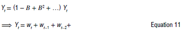
Y_i = (1 - L)^dX_t and

These concepts and equations were used in this study to forecast the values of TB incidence among under-5-year-old children for validation. However, autoregressive (AR) = φ(Z) and moving average (MA) = θ (z) characteristics polynomials are expressed as: φ(Z) = 1 - φ₁ z - φ₂ z² - ...- φ_ρZ^ρ and θ(Z) = 1 - θ₁ z - θ₂z² - ...- θ_qZ^q, The difference is taken d times until the original series becomes stationary, which is known as 'integrated'. In general, a d-th order difference can be written as: Y'_t = (1 - B)^dY_t, where B is the backshift operator. However, we created a basic univariate auto-ARIMA machine-learning model with a date-time feature in the model to generate the ARIMA model.

2. XGBoost model

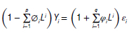
Extreme Gradient Boosting (XGBoost is a robust machine-learning system that employs gradient boosting decision tree algorithms. It assesses the significance of input features and predicts errors to make final predictions.^31-33 Originally developed by Chen Tianqi and Carlos Gestrin in 2011, XGBoost has seen continuous refinement and enhancement by various researchers.³⁴ In practice, it often requires multiple iterations to obtain sufficient accuracy.³⁵ XGBoost is a powerful gradient-boosting machine method.^36,37 The XGBoosting function can be written as:

where Y, is the observed value, Y_t^t-1 represents the predicted value from the last iteration, f_t represents the new function for learning models, x_i is the feature vector, n is the sample size, ø(f_t) is the regularisation term that controls model complexity, and l is the loss function that measures the difference between the label and the prediction in the previous phase to produce the output of the new tree.^32,38 For this study, an XGBoost model was created to specify a time-series model using boosting, aiming to enhance the modelling of residuals or errors related to exogenous regressors. The tuning parameter settings for this model included the number of randomly sampled predictors at each tree split within the ensemble. These arguments were specified with specific names during the model fitting process.

3. ETS model

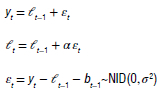
The ETS model, which utilises exponential smoothing within a state space framework, was employed as one of the predictive models for the time-series data. The algorithms used in the exponential smoothing techniques generated point forecasts from the state space model expressed as:

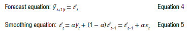
where ε_t = y_t - l_t-1 = y_t- y_t|t-1 is the residual at time t. The training data errors lead to the adjustment of the estimated level throughout the smoothing process. The model usually has a three-character string identification method using the framework terminology of Hyndman et al.³⁹ The residuals training additive errors e, is assumed to be normally distributed white noise with mean zero and variance σ² as:

When inserting these into the error correction equations for Holt's linear method, we get:

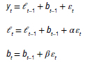
where β can be set as β = αβ*. Based on the classification, the method is fully automatic and only requires arguments for ETS time series.^40,41

4. Prophet model

The Prophet model, introduced by Facebook Inc. in 2017⁴², is designed for predicting time-series data characterised by significant seasonal patterns and multiple seasons of historical data⁴³. Prophet is known for its resilience in handling missing data and effectively managing outliers.⁴⁴ This model breaks down the time series into three primary components: the seasonal term S_t, the trend term 7,, and the residual term R_t:

In addition, to satisfy the needs of the actual scenario, the Prophet model integrates the effect of holidays h(t):

where g(t) describes a piecewise-linear trend (or 'growth term'), s(t) describes the various seasonal patterns, h(t) captures the holiday effects, and ε_t is a white noise error term.

In the Prophet model used, the first step was to model the time series with specified parameters. The second step was to set the weekly and daily seasonal components to True to improve the prediction argument results fitted in the model. The forecast was then obtained and the performance evaluated.

5. Time-series linear regression model

A time-series linear regression model uses a linear algorithm function from the parsnip R package workflow to model the trend and seasonality of the data. The function fits the regression model and machine-learning predictions using tidyverse R packages principles.⁴⁵ The linear model assumes a linear relationship that exists between the forecast and predictor variables, expressed as:

This indicates that the errors must have a mean of zero, or the forecasts are biased. The residuals must not be autocorrelated; if they are, the forecasts will be inefficient because the data contain more information that can be utilised. The residuals must be independent normal random variables with constant variance in order to create accurate inferences and prediction intervals. The trend is the slope of y_t = X_tβ + ε_t. The model uses predictions to generate new values for independent features. These feature lags are typically used in autoregressive models.

6. Multivariate Adaptive Regression Spline model

The MARS model was created by modifying the algorithm process to use a workflow that standardises the pre-processing of the features of MARS machine learning model. The algorithm automatically creates a piecewise linear model that captures the non-linear relationships in the data by assessing knots similar to step functions⁴⁶. The procedure evaluates each predictor from each of the data points as a knot and creates a linear regression model with the candidate feature(s). Considering non-linear, non-monotonic data where Y_t = f(X_t), the MARS procedure looks for a single point across the range of X_t values where two different linear relationships exist between Y_t and X_t achieve the smallest error (smallest SSE). This process continues until several knots are built to produce highly non-linear predictions, and the knots were used to fit a better relationship with our training data. After the full set of knots were established and identified, we removed those that did not significantly contribute to predictive accuracy.

7. Naïve random Walk

The NRW model in this study was based on an algorithm that assumes a variable Y_t takes a random step away from its previous value in each time period. These steps are independently and identically distributed in size (i.i.d.), represented as Y_t = Y_t-1 + w_t, where w_t is a discrete white noise series. To process the variable, the first difference is calculated, and the model's mean is applied. Additionally, a backward shift operator Β is applied to the NRW as follows:

And stepping back further:

This process was repeated until the end of the time series to get:

We used a workflow interface for adding pre-processing of the timeseries data into the algorithm functions of the NRW model.

8. Bayesian-ArIMA model

In this context, an ARIMA model was created similarly to Model 1, but with a Bayesian approach. The Bayesian structural regression algorithm was employed to specify a Bayesian structural time-series model before fitting to effectively handle unobserved components within time-series data and provides more accurate uncertainty estimates. This approach manages uncertainty more effectively by allowing the measurement of posterior uncertainty for individual components, control over component variances, and the incorporation of prior assumptions into the model. The model can be represented as follows:

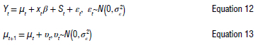
where μ_t is the unobserved trend, x_t represents a set of regressors, and S_t denotes seasonality. This technique does not rely on differencing, lags or moving averages. The model was created using the fit function from a stan algorithm of the bsts package in R to pre-process the time-series data.

Hybrid models

The proposed hybrid models used in this study were based on a combination of the RF model and the eight previously mentioned machine-learning models. The advantage of these hybrid models is that they leverage the strengths of both the RF model and a diverse set of complementary forecasting techniques. The hybrid approach is designed to capture both non-linear patterns of RF and probabilistic time-series forecasting strengths. This ensemble strategy improves robustness and generalisation, making it a strong candidate for forecasting childhood TB incidence, particularly for complex and noisy time-series data for which single models may not perform well consistently.

RF is a bagging-based ensemble method which constructs multiple de-correlated decision trees to improve predictive accuracy. It is widely regarded as a strong 'off-the-shelf' learning algorithm due to its reliable performance and minimal need for hyperparameter tuning. In this study, the RF model was implemented using the randomForest package in R, and variable importance metrics were examined to assess the contribution of different predictors. By combining RF with diverse forecasting techniques, we aimed to produce more stable and accurate TB incidence predictions over time.^9,18,47-49

In this analysis, the first measure involved permuting the TB data and recording the prediction error on the out-of-bag portion of the data using the mean squared error (MSE) for each tree in the regression classification. The MSE and variance were then calculated using the out-of-Bag-Error estimation. This procedure was used to assess the accuracy and robustness of the RF model. By using out-of-bag error estimation and calculating the MSE and variance, we obtained an unbiased measure of model performance without needing a separate validation set, helping ensure reliable predictions for TB incidence.

The model utilised two-thirds of the data for training and the remaining for testing to validate the trees. During the model creation, only one variable was randomly considered at each split, and a total of 500 trees were generated.

The results show a 72.9% increase in MSE for the model's variable importance and an 82.7% variance explained by the model. The analysis included plotting the error against the number of trees and also the absolute residual values against the probability distribution of random variables (Figure 1). This was done to determine the point at which the model's performance stabilises, helping to select an optimal number of trees and avoid overfitting. It was observed that, as more trees were added and averaged, there was a decreasing trend in the error.

 

 

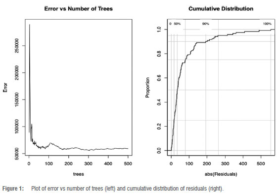
Errors were recorded using the MSE. Residuals from the RF model were calculated by subtracting the predicted TB values from the actual observed TB cases. These residuals represent the portion of the data not captured by the RF model. To improve forecasting accuracy, these residuals were then used as input for fitting various hybrid models, allowing the second model in each hybrid to learn and correct the errors made by the RF model. Then, hybrid models were employed to forecast TB cases for the years 2020, 2021 and 2022. Finally, the predictive accuracy of the single machine-learning models and the hybrid machine-learning models was compared to determine which model performed best in terms of predictive accuracy.

Accuracy metrics and model evaluation

We assessed the true model accuracy by comparing predicted values to actual values, using a range of performance metrics to precisely measure model accuracy. To comprehensively evaluate predictive performance and determine the best model, we employed three specific parameter metrics: mean absolute error (MAE), mean absolute scaled error (MASE) and root mean squared error (RMSE):

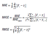
We evaluated the accuracy of each model using a test data set and then recalibrated to improve its forecasting accuracy across the entire data set.

Data analysis

The statistical analyses were conducted in RStudio (Version 4.1.0) and packages such as forecast, fpps, TTR, randomForest and bayesmodels were employed. These packages offered the essential tools to facilitate robust model-building and ensure the most accurate model configuration.

 

Results

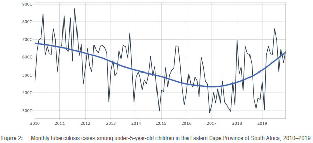
During the timeframe spanning from 2010 to 2019, a comprehensive analysis was conducted on a total of 120 cases of TB among children under the age of 5 years. Figure 2 shows the trajectory of TB incidents in under-5-year-old children in the Eastern Cape Province; a discernible upswing in reported TB cases can be seen between 2016 and 2019. It is noteworthy that the confirmed case counts fluctuated across months in a distinct pattern influenced by both annual seasonality and overarching long-term trends.

To facilitate effective model training and evaluation, the entire data set underwent a meticulous partitioning process, resulting in distinct training and testing subsets. To maintain a minimum of 100 samples for model training, the data set of 120 observations was split into 108 samples for training and 12 samples for testing (90/10 split). This ensured a sufficiently large training set while preserving a small but adequate testing set for model evaluation.

 

Comparison of model performance

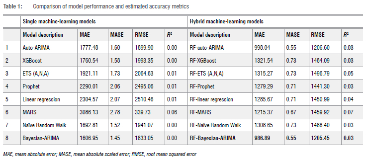
For the evaluation of model effectiveness, we employed MAE, MASE and RMSE to identify the optimal and most parsimonious model, marked by the lowest estimated accuracy values. Among the single models, the Bayesian-ARIMA model emerged as the best, showcasing the lowest MAE (1606.95), MASE (1.45) and RMSE (1833.05) values in contrast to the other models when forecasting the data. While all the models exhibited commendable performance, the RF-BARIMA model stood out as the best forecasting model, presenting the lowest MAE (986.89), MASE (0.55) and RMSE (1205.45) values (Table 1). Notably, the RF-BARIMA model demonstrated residuals that were independently distributed, further validating its reliability. The values for the models are near zero, not because the models are non-functional, but because of the high variance and weak linear signal in the target variable relative to the baseline (mean) model. In time-series forecasting, particularly with noisy or highly volatile data, often becomes misleading or uninformative, especially when the variance of the true values is large compared to the variance explained by the model. We have therefore prioritised more appropriate time-series metrics (MAE, RMSE, MASE) to assess model performance.

The analysis of the model outputs revealed that the hybrid BARIMA model provided better parameter estimates or predictions than the single BARIMA model. Specifically, the hybrid model was able to capture patterns or features in the TB incidence data more effectively. As a result, the values estimated by the hybrid model were more accurate, outperforming those generated by the single model. In comparison to the single model, the hybrid model showed enhanced parameter values: μ = 0.4122 ± 0.0497, σ = 1284.3384 ± 1.4460, ma = -0.7836 ± 0.0009, and sma = -0.0509 ± 0.0012, as outlined in Supplementary tables 1 and 2. This substantiates the potency of the hybrid approach in refining parameter estimations and ultimately bolstering forecasting precision.

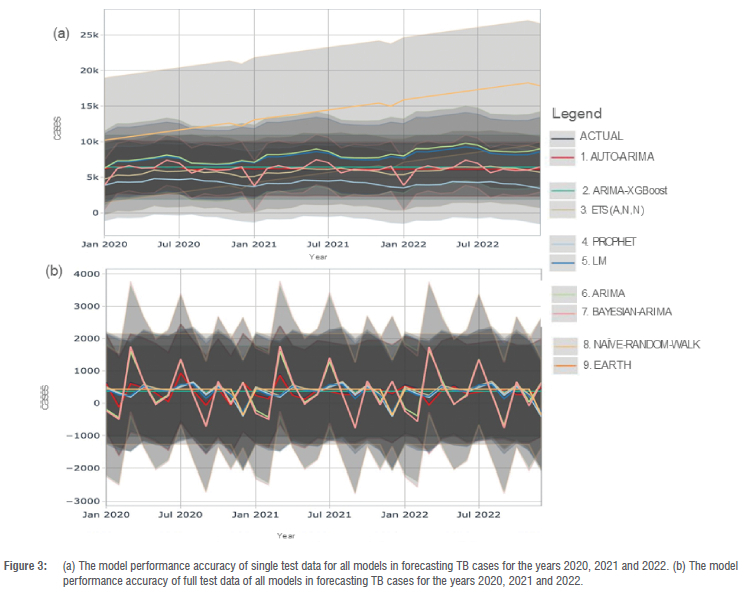
We assessed model performance by analysing the accuracy of the single models and combined models in forecasting TB cases among children under 5 years old from 2020 to 2022, as depicted in Figure 3. Examining the outcomes of the single models, the forecasting plot illustrates a consistent upward trajectory in TB incidence cases from the initial phase of the study's forecasting period in 2020 to its conclusion in 2022.

Remarkably, Model 7 emerged as the best performing model, boasting the most tightly bounded 80% confidence interval, which attests to the model's exceptional forecasting precision. Model 2 also demonstrated commendable performance, largely attributed to the judiciously specified parameters of its XGBoost components, but the model's accuracy is suboptimal.

Model 3's performance closely rivalled the efficacy of Model 2, albeit with a marginally broader test error confidence interval. In contrast, Models 4, 5 and 9 exhibited a tendency to overshoot the local trend due to the inherent linear trend components that failed to account for change points. Similarly, Models 1, 6 and 8 overfitted the local trend, primarily due to the underexplored adjustment of the number of change points. These observations, succinctly depicted in Figure 3a, underscore the nuanced interplay of model components and parameters in shaping the accuracy and precision of TB incidence forecasts among children under 5 years old.

The accuracy of the full models (i.e. all predictors and components) in forecasting TB cases among children under 5 years old from 2020 to 2022 is illustrated in Figure 3b. The figure depicts a subtle upward trend in TB incidence cases at the onset of the forecasting period in 2020, followed by slight declines in TB cases during 2021 and 2022. Notably, minimal differences were observed when comparing the performance of the models in predicting the trajectory of TB incidence among children under 5.

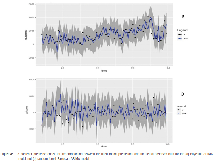
The posterior predictive performance of the RF-BARIMA model was better than that of the Bayesian-ARIMA model, which was employed to fit the data and validate the compatibility of the fitted model with actual observations (as illustrated in Figure 4). The visual representation of the model plot distinctly demonstrates the consistency and adequacy of the model's compatibility in describing the observed data across multiple years. Within this depiction, the black dot signifies the distribution of observed outcomes, denoted as "y", while the array of blue lines represents the residual estimates derived from the posterior predictive distribution, labelled as "y". Notably, the encompassing grey area delineates the expected 95% credible interval of the observations falling within the predicted 95% credible intervals, provided that the model is aptly suited to depict the data set's characteristics.

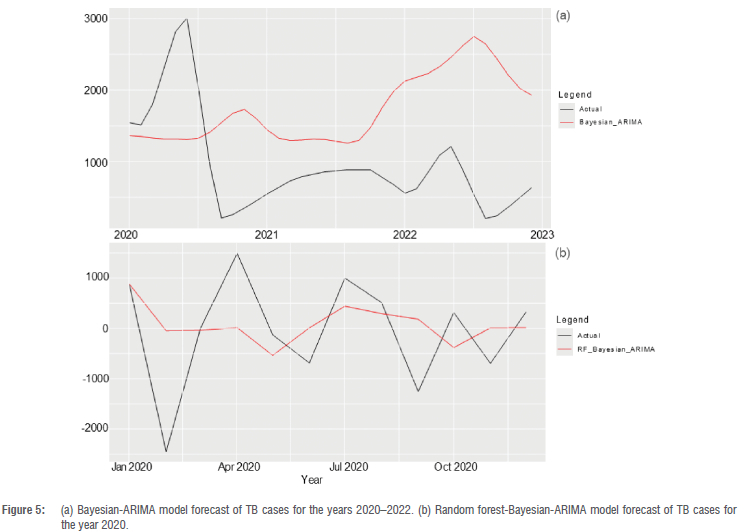
The RF-BARIMA and Bayesian-ARIMA models were compared in TB cases forecasting among children under 5 years from 2020 to 2022 (as illustrated in Figure 5). Notably, the RF-BARIMA model exhibited the highest accuracy in forecasting performance with an MAE of 986.89, MASE of 0.55 and RMSE of 1205.45, compared with the Bayesian-ARIMA model with an MAE of 1606.95, MASE of 1.45 and RMSE of 1833.05. These results show the improved forecasting performance of the hybrid RF-BARIMA model. The plot shows a decreasing temporal pattern in TB incidence cases at the outset of the 2020 forecast period, followed by an increase around mid-2021, and another decline towards the end of the forecasting year.

 

Discussion

Before the COVID-19 pandemic, TB cases among children under 5 showed alternating patterns of increase and decrease from 2017 to 2019. By analysing this trendline, we observed a series of lower highs (indicating a downtrend) and higher lows (indicating an uptrend), which created a resistance level that could influence future TB case trends. The TB temporal analysis shows high reported rates of TB incidence among under-5-year-old children in this study, which can be explained by the prevalence of infectious TB in adults, social interactions between adults and children, and the ventilation conditions in domestic settings.^50-52

This study shows that not all models predicted childhood TB cases with equal accuracy. Each model demonstrated different levels of prediction error, with the RF-Bayesian-ARIMA hybrid model consistently outperforming all others across multiple error metrics. This suggests that, while some models were able to reasonably forecast childhood TB incidence, others showed relatively high prediction errors and were less reliable - a result which aligns with previous studies.^9,18,47,48 Other studies have shown the superiority of machine-learning hybrid models in accurately forecasting TB cases.^5,9,53 Infectious disease data often exhibit various linear and non-linear features, making single models inadequate for modelling such data. Hybrid models have consistently proven to be the most suitable choice for estimating such complex data.⁴⁹

The estimated incidence of TB cases in the Eastern Cape was 328 per 100 000 among children under 15 years old in 2020; 7% of cases were among children under 5 years.¹ Children are at greater risk of contracting TB.⁵⁴ Our study's forecast for 2022 predicts an average of 41.22% TB cases per month, based on a sample size of 4054 TB cases in the Eastern Cape Province. This forecast indicates a future decrease of 1671 TB cases among children under 5 years old. These findings align with a similar study conducted in two Kenyan counties that projected Tb cases among children under 15 years old and found that the estimated TB cases were slightly lower than the general population in Kenya.⁹

The findings of this study show a slight declining trend in TB incidence cases at the start of the forecasting period in 2020, followed by slight increases in TB cases in 2021 and 2022. These trends align with findings from a WHO report which suggested that the number of TB cases could rise in 2021 and 2022, largely due to the impact of the COVID-19 pandemic.¹ This prediction encompasses not only the general population but also includes cases among children under 15 years of age.

Our study shows that TB incidence cases among children under the age of 5 follow a seasonal pattern, with peaks occurring in June, July and August, followed by a decrease over the rest of the year till in the year. This observation is consistent with those of previous studies that also found seasonal variations contributing to TB infections^55,56, although another study did not find any association between TB infections and seasonal trends.⁵⁷ Our study's findings suggesting a connection between TB infections in children and seasons can be explained by the impact of seasonal patterns on TB transmission. Children tend to spend more time indoors during the winter season, which is conducive to tB growth due to factors like overcrowding, increased humidity and reduced air circulation.

Under-5-year-old children, especially during mid-winter, have been reported to have low vitamin D levels.⁵⁸ This deficiency could make these children more susceptible to TB infections during winter, thus potentially contributing to the observed seasonal pattern of TB infections. While children can contract TB at any age, it is most prevalent among those aged 1-4 years, likely due to their underdeveloped immune systems. The highest TB notification rate in South Africa's Western Cape Province was reported for children in the 0-2-year age group.⁵⁹ Hospital studies indicate that extrapulmonary TB is more common in children than is pulmonary TB, and misdiagnosis is a recurring issue.⁶⁰

 

Limitations

This study relied on data collected and reported through the Eastern Cape ERTNET system, and, therefore, we had no control over the data's quality and accuracy. However, it was assumed that, as the data had been submitted to the system, the health facilities in the Province had followed all relevant protocols to ensure data quality.

We used data from 2010 to 2019, consisting of 120 monthly aggregated TB cases in children under 5 years old. Deep learning and machine-learning algorithms typically require a large volume of data to learn effectively. Consequently, the provided data set may not have been sufficient to allow the algorithm to learn more efficiently.

It is important to note that out-of-bag error estimation can have limitations in small or highly imbalanced data sets, such as the one used in this study, where the number of training samples (108) is relatively small compared to the number of trees in the RF model.

 

Conclusion

The RF-BARIMA model performed best in predicting TB cases among children under 5 years. Our findings highlight the persistent under-reporting of TB cases in this age group, suggesting that the actual incidence might be higher than previously estimated. To address this issue, there is a need to re-evaluate the TB monitoring framework data to identify existing gaps and urgently allocate resources to the national TB programme.

Additionally, our study shows that TB infections among children under 5 years are influenced by seasonal patterns. This calls for increased investment in TB surveillance, screening and diagnostic efforts during specific months of the year to curb the spread of infection during peak seasons.

 

Data availability

The data supporting the results of this study are available upon request to the corresponding author. Detailed procedures and codes utilised in our analysis are conveniently accessible at https://github.com/azizadeboye/rf-barima-tb-forecasting-south-africa/. This repository contains the requisite codes to replicate and further investigate our analytical approach.

 

Declarations

We have no competing interests to declare. We have no AI or LLM use to declare. This study was approved by the Eastern Cape Department of Health (approval number: EC_20210_014) and the Research Ethics Committee of the University of Fort Hare (approval number: REC-100118-054). Written permission was also received from the office of the District Manager of the Amathole Health District to access the relevant health data used in this study.

 

Authors' contributions

A.A.: Conceptualisation, methodology, investigation, sample analysis, formal analysis, validation, data curation, writing - original draft, writing - review and editing. G.O.: Conceptualisation, methodology, investigation, formal analysis, validation, writing - original draft, writing - review and editing. R.M.: Conceptualisation, methodology, investigation, sample analysis, formal analysis, validation, writing - original draft, writing - review and editing. J.N.: Conceptualisation, methodology, sample analysis, validation, writing - original draft. All authors read and approved the final manuscript.

 

References

1. World Health Organization (WHO). Global tuberculosis report 2022. Geneva: WHO: 2022. Available from: https://www.who.int/publications/i/item/9789240061729        [ Links ]

2. Marais BJ, Verkuijl S, Casenghi M, Triasih R, Hesseling AC, Mandalakas AM, et al. Paediatric tuberculosis - new advances to close persistent gaps. Int J Infect Dis. 2021;113(Suppl 1):S63-S67. https://doi.org/10.1016/j.ijid.2021.02.003        [ Links ]

3. Walters E, van der Zalm MM, Demers AM, Whitelaw A, Palmer M, Bosch C, et al. Specimen pooling as a diagnostic strategy for microbiologic confirmation in children with intrathoracic tuberculosis. Pediatr Infect Dis J. 2019;38(6):e128-e131. https://doi.org/10.1097/INF.0000000000002240        [ Links ]

4. Ioos V Cordel H, Bonnet M. Alternative sputum collection methods for diagnosis of childhood intrathoracic tuberculosis: A systematic literature review. Arch Dis Child. 2019;104:629-635. https://doi.org/10.1136/archdischild-2018-315453        [ Links ]

5. Maipan-Uku JY, Cavus N. Forecasting tuberculosis incidence: A review of time series and machine learning models for prediction and eradication strategies. Int J Environ Health Res. 2024;35(3):645-660. https://doi.org/10.1080/09603123.2024.2368137        [ Links ]

6. Karmani P, Chandio AA, Korejo IA, Samuel OW, Aborokbah M. Machine learning based tuberculosis (ML-TB) health predictor model: Early TB health disease prediction with ML models for prevention in developing countries. PeerJ Comput Sci. 2024;10, e2397. https://doi.org/10.7717/peerj-cs.2397        [ Links ]

7. Marcy O, Borand L, Ung V, Tejiokem M, Huu KT, Chau VD, et al. A treatment-decision score for HIV-infected children with suspected tuberculosis. Pediatrics. 2019;144(3), e20182065. https://doi.org/10.1542/peds.2018-2065        [ Links ]

8. Gunasekera KS, Walters E, van der Zalm MM, Palmer M, Warren JL, Hesseling AC, et al. Development of a treatment-decision algorithm for human immunodeficiency virus-uninfected children evaluated for pulmonary tuberculosis. Clin Infect Dis. 2021;73(4):e904-e912. https://doi.org/10.1093/cid/ciab018        [ Links ]

9. Siamba S, Otieno A, Koech J. Application of ARIMA, and hybrid ARIMA models in predicting and forecasting tuberculosis incidences among children in Homa Bay and Turkana Counties, Kenya. PLOS Digit Health. 2023;2(2), e0000084. https://doi.org/10.1371/journal.pdig.0000084        [ Links ]

10. Abdualgalil B, Abraham S, Ismael WM, George D. Modeling and forecasting tuberculosis cases using machine learning and deep learning approaches: A comparative study. In: Goswami S, Barara IS, Goje A, Mohan C, Bruckstein AM, editors. Data management, analytics and innovation. Singapore: Springer; 2023. p. 157-171. https://doi.org/10.1007/978-981-19-2600-6_11        [ Links ]

11. World Health Organization (WHO). WHO operational handbook on tuberculosis: Module 5: Management of tuberculosis in children and adolescents. Geneva: WHO; 2022 [cited 2024 Apr 03]. Available from: https://www.who.int/publications/i/item/9789240046832        [ Links ]

12. Zhao YF, Shou MH, Wang ZX. Prediction of the number of patients infected with COVID-19 based on rolling grey Verhulst models. Int J Environ Res Public Health. 2020;17(12), Art. #4582. https://doi.org/10.3390/ijerph17124582        [ Links ]

13. Guan P, Wu W, Huang D. Trends of reported human brucellosis cases in mainland China from 2007 to 2017: An exponential smoothing time series analysis. Environ Health Prev Med. 2018;23, Art. #23. https://doi.org/10.1186/s12199-018-0712-5        [ Links ]

14. Zhang YQ, Li XX, Li WB, Jiang JG, Zhang GL, Zhuang et al. Analysis and predication of tuberculosis registration rates in Henan Province, China: An exponential smoothing model study. Infect Dis Poverty. 2020;9, Art. #123. https://doi.org/10.1186/s40249-020-00742-y        [ Links ]

15. Martínez-Bello DA, López-Quílez A, Torres-Prieto A. Bayesian dynamic modeling of time series of dengue disease case counts. PLoS Negl Trop Dis. 2017;11(7), e0005696. https://doi.org/10.1371/journal.pntd.0005696        [ Links ]

16. Wang Y, Xu C, Zhang S, Wang Z, Zhu Y, Yuan J. Temporal trends analysis of human brucellosis incidence in mainland China from 2004 to 2018. Sci Rep. 2018;8, Art. #15901. https://doi.org/10.1038/s41598-018-33165-9        [ Links ]

17. Wang Xu C, Li Y, Wu W, Gui L, Ren J, et al. An advanced data-driven hybrid model of SARIMA-NNNAR for tuberculosis incidence time series forecasting in Qinghai Province, China. Infect Drug Resist. 2020;13:867-880. https://doi.org/10.2147/IDR.S232854        [ Links ]

18. Azeez A, Obaromi D, Odeyemi A, Ndege J, Muntabayi R. Seasonality and trend forecasting of tuberculosis prevalence data in Eastern Cape, South Africa, using a hybrid model. Int J Environ Res Public Health. 2016;13(8), Art. #757. https://doi.org/10.3390/ijerph13080757        [ Links ]

19. Li Z, Wang Z, Song H, Liu Q, He B, Shi P et al. Application of a hybrid model in predicting the incidence of tuberculosis in a Chinese population. Infect Drug Resist. 2019;12:1011-1020. https://doi.org/10.2147/IDR.S190418        [ Links ]

20. Wang Y, Xu C, Wang Z, Zhang S, Zhu Y, Yuan J. Time series modeling of pertussis incidence in China from 2004 to 2018 with a novel wavelet based SARIMA-NAR hybrid model. PLoS One. 2018;13, e0208404. https://doi.org/10.1371/journal.pone.0208404        [ Links ]

21. Wang Y, Xu C, Zhang S, Wang Z, Yang L, Zhu Y, et al. Temporal trends analysis of tuberculosis morbidity in mainland China from 1997 to 2025 using a new SARIMA-NARNNX hybrid model. BMJ Open. 2019;9, e024409. https://doi.org/10.1136/bmjopen-2018-024409        [ Links ]

22. Novak J, McGarvie S, Garcia BE. A Bayesian model for forecasting hierarchically structured time series [preprint].arXiv. Version 1. 2017. Available from: https://doi.org/10.48550/ARXIV.1711.04738        [ Links ]

23. Zeng Z, Li M. Bayesian median autoregression for robust time series forecasting. Int J Forecast. 2021;37:1000-1010. https://doi.org/10.1016/j.ijforecast.2020.11.002        [ Links ]

24. Vosseler A, Weber E. Forecasting seasonal time series data: A Bayesian model averaging approach. Comput Stat. 2018;33:1733-1765. https://doi.org/10.1007/s00180-018-0801-3        [ Links ]

25. Xiao Q, Chaoqin C, Li Z. Time series prediction using dynamic Bayesian network. Optik. 2017;135:98-103. https://doi.org/10.1016/j.ijleo.2017.01.073        [ Links ]

26. Rodriguez A, Puggioni G. Mixed frequency models: Bayesian approaches to estimation and prediction. Int J Forecast. 2010;26(2):293-311. https://doi.org/10.1016/j.ijforecast.2010.01.009        [ Links ]

27. Ganics G, Odendahl F. Bayesian VAR forecasts, survey information, and structural change in the euro area. Int J Forecast. 2021;37(2):971-999. https://doi.org/10.1016/j.ijforecast.2020.11.001        [ Links ]

28. Zhang AY, Lu M, Kong D, Yang J. Bayesian time series forecasting with change point and anomaly detection. Paper presented at: ICLR 2018 Conference; 2018 Apr 30 - May 03; Vancouver, Canada.         [ Links ]

29. van der Heijden M, Velikova M, Lucas PJF. Learning Bayesian networks for clinical time series analysis. J Biomed Inform. 2014;48:94-105. https://doi.org/10.1016/j.jbi.2013.12.007        [ Links ]

30. Panagiotelis A, Smith M. Bayesian density forecasting of intraday electricity prices using multivariate skew t distributions. Int J Forecast. 2008;24(4):710-727. https://doi.org/10.1016/j.ijforecast.2008.08.009        [ Links ]

31. Zheng Y, Zhu Y, Ji M, Wang R, Liu X, Zhang M, et al. A learning-based model to evaluate hospitalization priority in COVID-19 pandemics. Patterns. 2020;1(6), Art. #100092. https://doi.org/10.1016/j.patter.2020.100092        [ Links ]

32. Lv CX, An SY, Qiao BJ, Wu W. Time series analysis of hemorrhagic fever with renal syndrome in mainland China by using an XGBoost forecasting model. BMC Infect Dis. 2021;21, Art. #839. https://doi.org/10.1186/s12879-021-06503-y        [ Links ]

33. Hu CA, Chen CM, Fang YC, Liang SJ, Wang HC, Fang WF, et al. Using a machine learning approach to predict mortality in critically ill influenza patients: A cross-sectional retrospective multicentre study in Taiwan. BMJ Open. 2020;10(2), e033898. https://doi.org/10.1136/bmjopen-2019-033898        [ Links ]

34. Li W, Yin Y, Quan X, Zhang H. Gene expression value prediction based on XGBoost algorithm. Front Genet. 2019;10, Art. #1077. https://doi.org/10.3389/fgene.2019.01077        [ Links ]

35. Wang T, Liu J, Zhou Y, Cui F, Huang Z, Wang L, et al. Prevalence of hemorrhagic fever with renal syndrome in Yiyuan County, China, 2005-2014. BMC Infect Dis. 2015;16, Art. #69. https://doi.org/10.1186/s12879-016-1404-7        [ Links ]

36. Shrivastav LK, Jha SK. A gradient boosting machine learning approach in modeling the impact of temperature and humidity on the transmission rate of COVID-19 in India. Appl Intell. 2021;51:2727-2739. https://doi.org/10.1007/s10489-020-01997-6        [ Links ]

37. Babajide Mustapha I, Saeed F. Bioactive molecule prediction using extreme gradient boosting. Molecules. 2016;21(8), Art. #983. https://doi.org/10.3390/molecules21080983        [ Links ]

38. Nishio M, Nishizawa M, Sugiyama O, Kojima R, Yakami M, Kuroda T, et al. Computer-aided diagnosis of lung nodule using gradient tree boosting and Bayesian optimization. PLoS One. 2018;13(4), e0195875. https://doi.org/10.1371/journal.pone.0195875        [ Links ]

39. Hyndman RJ, Koehler AB, Snyder RD, Grose S. A state space framework for automatic forecasting using exponential smoothing methods. Int J Forecast. 2002;18(3):439-454. https://doi.org/10.1016/S0169-2070(01)00110-8        [ Links ]

40. Hyndman RJ, Akram M, Archibald BC. The admissible parameter space for exponential smoothing models. Ann Inst Stat Math. 2008;60:407-426. https://doi.org/10.1007/s10463-006-0109-x        [ Links ]

41. Hyndman R, Koehler A, Ord K, Snyder R. Forecasting with exponential smoothing. Berlin: Springer; 2008. https://doi.org/10.1007/978-3-540-71918-2        [ Links ]

42. Taylor SJ, Letham B. Forecasting at scale. Am Stat. 2018;72(1):37-45. https://doi.org/10.1080/00031305.2017.1380080        [ Links ]

43. Xie C, Wen H, Yang W, Cai J, Zhang P, Wu R, et al. Trend analysis and forecast of daily reported incidence of hand, foot and mouth disease in Hubei, China by Prophet model. Sci Rep. 2021;11, Art. #1445. https://doi.org/10.1038/s41598-021-81100-2        [ Links ]

44. Rostami-Tabar B, Rendon-Sanchez JF. Forecasting COVID-19 daily cases using phone call data. Appl Soft Comput. 2021;100, Art. #106932. https://doi.org/10.1016/j.asoc.2020.106932        [ Links ]

45. Kuhn M, Vaughan D. parsnip: A common API to modeling and analysis functions. R package version 1.3.3. Vienna: R Foundation for Statistical Computing; 2025. https://github.com/tidymodels/parsnip        [ Links ]

46. Boehmke B, Greenwell BM. Hands-on machine learning with R. New York: Chapman and Hall/CRC; 2019. https://doi.org/10.1201/9780367816377        [ Links ]

47. Cao S, Wang F, Tam W, Tse LA, Kim JH, Liu J, et al. A hybrid seasonal prediction model for tuberculosis incidence in China. BMC Med Inform Decis Mak. 2013;13, Art. #56. https://doi.org/10.1186/1472-6947-13-56        [ Links ]

48. Zhou L, Xia J, Yu L, Wang Y, Shi Y, Cai S, et al. Using a hybrid model to forecast the prevalence of schistosomiasis in humans. Int J Environ Res Public Health. 2016;13(4), Art. #355. https://doi.org/10.3390/ijerph13040355        [ Links ]

49. Chakraborty T, Chakraborty AK, Biswas M, Banerjee S, Bhattacharya S. Unemployment rate forecasting: A hybrid approach. Comput Econ. 2021; 57:183-201. https://doi.org/10.1007/s10614-020-10040-2        [ Links ]

50. Shanaube K, Sismanidis C, Ayles H, Beyers N, Schaap A, Lawrence KA, et al. Annual risk of tuberculous infection using different methods in communities with a high prevalence of TB and HIV in Zambia and South Africa. PLoS One. 2009;4(11), e7749. https://doi.org/10.1371/journal.pone.0007749        [ Links ]

51. Wood R, Liang H, Wu H, Middelkoop K, Oni T, Rangaka MX, et al. Changing prevalence of tuberculosis infection with increasing age in high-burden townships in South Africa. Int J Tuberc Lung Dis. 2020;14(4):406-412.         [ Links ]

52. Middelkoop K, Bekker LG, Morrow C, Zwane E, Wood R. Childhood tuberculosis infection and disease: A spatial and temporal transmission analysis in a South African township. S Afr Med J. 2009;99(10):738-743.         [ Links ]

53. Mate Landry G, Nsimba Malumba R, Balanganayi Kabutakapua FC, Boluma Mangata B. Performance comparison of classical algorithms and deep neural networks for tuberculosis prediction. J Techno Nusa Mandiri. 2024;21(2):126-133. https://doi.org/10.33480/techno.v21i2.5609        [ Links ]

54. Negin J, Abimbola S, Marais BJ. Tuberculosis among older adults - time to take notice. Int J Infect Dis. 2015;32:135-137. https://doi.org/10.1016/j.ijid.2014.11.018        [ Links ]

55. Kirolos A, Thindwa D, Khundi M, Burke RM, Henrion MYR, Nakamura I, et al. Tuberculosis case notifications in Malawi have strong seasonal and weather-related trends. Sci Rep. 2021;11, Art. #4621. https://doi.org/10.1038/s41598-021-84124-w        [ Links ]

56. Bodena D, Ataro Z, Tesfa T. Trend analysis and seasonality of tuberculosis among patients at the Hiwot Fana specialized University Hospital, Eastern Ethiopia: A retrospective study. Risk Manag Healthc Policy. 2019;12:297-305. https://doi.org/10.2147/RMHRS228659        [ Links ]

57. Jaganath D, Wobudeya E, Sekadde MP, Nsangi B, Haq H, Cattamanchi A, et al. Seasonality of childhood tuberculosis cases in Kampala, Uganda, 20102015. RLoS One. 2019;14(4), e0214555. https://doi.org/10.1371/journal.pone.0214555        [ Links ]

58. Graham D, Kira G, Conaglen J, McLennan S, Rush E. Vitamin D status of Year 3 children and supplementation through schools with fortified milk. Public Health Nutr. 2009;12(12):2329-2334. https://doi.org/10.1017/S1368980008004357        [ Links ]

59. Fares A. Seasonality of tuberculosis. J Glob Infect Dis. 2011;3:46-55. https://doi.org/10.4103/0974-777X.77296        [ Links ]

60. Datta M, Swaminathan S. Global aspects of tuberculosis in children. Raediatr Respir Rev. 2001;2(2):91-96. https://doi.org/10.1053/prrv.2000.0115        [ Links ]

 

 

Correspondence:
Adeboye Azeez
Email: azizadeboye@gmail.com

Received: 16 Sep. 2023
Revised: 29 Jan. 2025
Accepted: 03 July 2025
Published: 26 Nov. 2025

 

 

Editors: Ebrahim Momoniat, Rodney Medupe, Stefan Lotz
Funding: None

 

 

Supplementary Data

The supplementary data is available in pdf: [Supplementary data]