RESEARCH ARTICLE

 

Modeling tropospheric ozone and particulate matter in Tunis, Tunisia using generalized additive model

 

 

Zouhour Hammouda^{I, II}; Leila Hedhili Zaier^I; Nadège Blond^III

^IInstitut Supérieur de Gestion, Tunis, Tunisia
^IIEsprit School of Engineering, Tunis, Tunisia
^IIILaboratoire Image Ville Environnement, UMR 7362CNRS/UDS, 3, rue de l'Argonne, 67000 Strasbourg, France

 

 

---

ABSTRACT

The main purpose of this paper is to analyze the sensitivity of tropospheric ozone and particulate matter concentrations to changes in local scale meteorology with the aid of meteorological variables (wind speed, wind direction, relative humidity, solar radiation and temperature) and intensity of traffic using hourly concentration of NO_X, which are measured in three different locations in Tunis, (i.e. Gazela, Mannouba and Bab Aliwa). In order to quantify the impact of meteorological conditions and precursor concentrations on air pollution, a general model was developed where the logarithm of the hourly concentrations of O₃ and PM₁₀ were modeled as a sum of non-linear functions using the framework of Generalized Additive Models (GAMs). Partial effects of each predictor are presented. We obtain a good fit with R² = 85% for the response variable O₃ at Bab Aliwa station. Results show the aggregate impact of meteorological variables in the models explained 29% of the variance in PM₁₀ and 41% in O₃. This indicates that local meteorological condition is an active driver of air quality in Tunis. The time variables (hour of the day, day of the week and month) also have an effect. This is especially true for the time variable "month" that contributes significantly to the description of the study area.

Keywords: Air pollution, Particulate Matter, Tropospheric Ozone, GAM, meteorology, traffic

---

 

 

Introduction

Nowadays, it is well known that air pollution and its impact on human health have become a primary topic in atmosphere research. A good number of epidemiological studies have demonstrated the strong link between atmospheric pollution and daily deaths and hospitalizations of pulmonary and cardiac diseases (Sinharay et al., 2017; Bourdrel et al., 2017). Tunisia is a beautiful country with diverse, complex geography and is located between the Mediterranean coast and the Saharan region. This location together with a diversity of air pollution sources (e.g. traffic, industrial, dust) leads to exceedances of air quality guideline values recommended by the World Health Organization (WHO, 2016). Tunisia reports high annual mean concentrations of PM_2.5 and PM₁₀, which should not exceed 10 and 20 μg.m^-3, respectively (WHO, 2016). Accelerated growth in emission sources of air pollutants in most important Tunisian cities like Tunis, Sfax and Gabes (Melki, 2007; Bouchlaghem and Nsom, 2012) now cause an urgent need to adopt specific policies in managing air pollution.

Air pollution modeling is an integral part of air pollution management and policy (Karaca et al., 2006; Saffarini and Odat, 2008). Previous air quality studies conducted in Tunisia mainly focused on the physical characteristics, correlations between pollutants, the sources of PM₁₀ and forecasting air quality (Melki, 2007; Bouchlaghem et al., 2009; Ayari, Nouira and Trabelsi, 2012; Calzolai et al., 2015). A few investigations focusing on the interplay between meteorology and air quality has been done in Tunisia. The study conducted in Tunis (Melki, 2007) presents the role of the temperature inversions, which determine the majority of the highest pollution levels in the north of the country. They used multiple linear regressions to evaluate the statistic dependence between the ozone concentrations and the weather conditions. According to Bouchlaghem et al. (2009), some sea breeze events are responsible for air quality. Their result shows that under these circumstances, the nearby power plant is responsible for air quality degradation in the region of Sousse (the East central part of Tunisia). Bouchlaghem and Nsom (2012) highlighted the influence of the Saharan dust on PM₁₀ concentrations. They concluded that PM₁₀ concentrations on days with Saharan dust contributions are higher than the average daily value with the absence of this phenomenon. In sum, no study has as yet dealt with the relationship between particulate matter and ozone concentrations and meteorological conditions in Tunisia based on the use of a non-linear statistical approach.

Generalized Additive Model, as an extension of Generalized Linear Model, has been employed in few studies for modeling pollutant concentrations, especially PM₁₀ (Taheri Shahraiyni et al., 2015) and O₃ (Ma et al., 2020). As a statistical tool that is able to simulate non-linear relationships by smoothing input variables (Hastie and Tibshirani, 1990), Generalized Additive Models (GAM) have been used in many environmental issues and recent studies (Ma et al., 2020; Yang et al., 2020). In the last two decades, this statistical approach has been used as a standard analytic tool in time-series studies of air pollution and human health (He, Mazumdar and Arena, 2005; Dehghan et al., 2018; Ravindra et al., 2019).

GAM models delivered good performance and can be equivalent to those of other methods such as neural networks (Schlink et al., 2003). Aldrin and Haff (2005) used meteorological predictors in order to model PM₁₀, PM₂₅ and the difference between PM₁₀ and PM₂₅ mass concentrations, and their models gave a reasonably good fit in terms of the squared correlation coefficient with 72% and 80% for PM₁₀ and NO_X, respectively. Pearce et al. (2011) noted the influence of local-scale meteorological conditions on air quality in Melbourne (Australia). Munir et al. (2013) offered a new GAM to predict daily concentrations of PM₁₀ in Makkah using lag PM₁₀ concentrations. This model showed the vital role of meteorological variables and traffic related air pollutants in describing the variations of the PM₁₀ concentrations. Again based on GAM analysis, Belusic, Herceg-Bulic and Bencetic Klaic (2015) employed the novel GAM approach to quantify the influence of local meteorology on air quality in Zagreb, Croatia. This study confirmed the well-known impact of wind direction and speed in variations of air pollution.

The objective of this study is to investigate the magnitude in which pollutant concentrations respond to measures of local meteorology and temporal variables in Tunis. Statistical models were developed for hourly mean PM₁₀ and O₃ concentrations for three sites of Tunis in order to quantify the impact of meteorology on PM₁₀ and O₃ levels. The paper is organized as follows: The Materials and methods section provides information on our data sources and data-handling methodology. Then it presents the description of the proposed methods and a brief introduction to Generalized Additive Models. The Results and discussion section discusses the findings, highlights the most important results and details a statistical evaluation of the model. Finally, we conclude the work in the Conclusions.

 

Materials and methods

Site description and sample collection

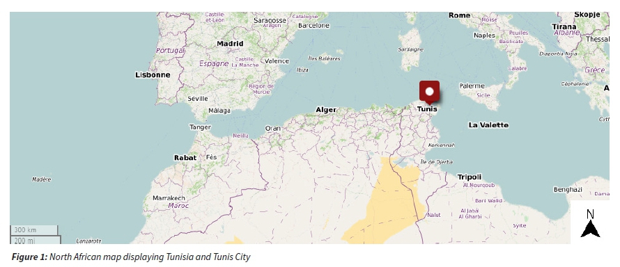
The study area is located in the metropolis of the Greater Tunis region, which consists of four governorates: Tunis, Ariana, Manouba and Ben Arous. The area of the Greater Tunis is 300,000 hectares, with a population of 2.5 million. This city contributes 30% to the total pollution of the country (INS, 2014) (Fig. 1).Three urban and suburban monitoring stations (i.e. Bab Aliwa, Gazela and Mannouba) were selected for this study (Fig. 2). These stations are located in three governorates: Tunis, Ariana and Mannouba.

Tunis City (capital of Tunisia) is located in the North part of Tunisia (36°49' N, 10°11' E). The urban area (1 056 247 inhabitants) is about 346 km² surface. The sampling site "Bab Aliwa" is classified as urban, is located in the vicinity of one of Tunis's major traffic avenues and is near to central bus station and the largest cemetery in the country.

Ariana is also located in the North part of Tunisia (36° 51' N 10° 11' E). Its urban area accounts about 576 088 inhabitants. The measurement station sample "Gazela" is classified as urban and is mainly influenced by residential, traffic, and commercial activities.

Mannouba is located in the center of the northern governorates (36° 48' N 10° 5' E). The urban area (379 518 inhabitants) is about 1 137 km² surface. The sampling site "Mannouba" is suburban and it is known for its typically agricultural and industrial character.

The data set used consists of pollution data for the period from 01/01/2008 to 31/12/2009, with corresponding measurements of meteorological conditions provided by "Agence Nationale de Protection de l'Environnement" (ANPE). This period was chosen because it is the only one with few missing values (< 7%). At each site, air pollution is measured with standards methods used in Tunisia. PM₁₀ and O₃ instruments are designed by Teledyne Advanced Pollution Instrumentation Company (http://www.teledyneapi.com). Levels of PM₁₀ were calculated by means of automatic beta radiation attenuation monitors. For O₃, the Teledyne model used is 400A. Data processing techniques and standard methods are described in the analyser instruction manuals. Additionally, all stations were equipped with automatic weather monitoring. All data series were collected hourly. Due to measurement errors, a few negative pollutant concentration values occasionally appeared in the raw data. These values cause problems because pollution data are modelled at log-scale (Aldrin and Haff, 2005) and have been replaced by the minimum observation in the data (1 ppb for NO_X and O₃ and 1 μg.m^-3 for PM₁₀). The limited sensitivity of the measurement instruments caused many observed zero values (about 0.05% on average), which were considered as erroneous data.

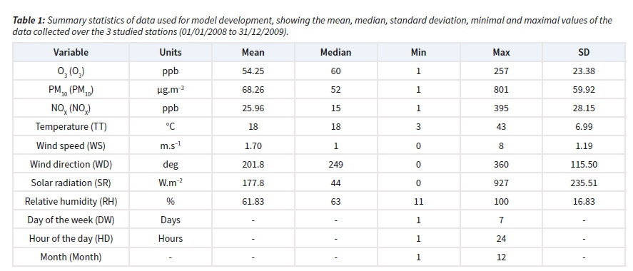
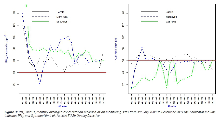
Table 1 presents a basic statistical overview of air pollution and meteorological variable values after the application of the data quality control process. Fig. 3 shows the average seasonal evolution of PM₁₀ (from January 2008 to December 2009) in the studied regions. We note different behavior at the various sites with very high levels compared to the PM₁₀ annual limit of the 2008 EU Air Quality Directive (40 μg.m^-3). The right-hand plot indicates that average seasonal evolution of O₃ is around the O₃ maximum daily 8-hour mean limit (60 ppb) of the 2008 EU Air Quality Directive (Directive, 2008), except for Gazela site, an overshoot was observed. So, pollution levels can be differentiated by geographical area. In Algeria, the north African country like Tunisia, the modeling results of Belhout et al. (2018) show that the Algerian annual average limit for PM₁₀ (80 μg.m^-3) has been exceeded in some Algiers areas; by consequence, air quality guidelines fixed by the WHO (20 μg.nr³), (WHO, 2006) and the European Union (EU) (40 μg.m^-3) for PM₁₀ are also exceeded. Rahal et al. (2014) found that significant pollutant releases in the study area are located at hyper-centre and at centre of the Wilaya of Algiers. Many sites in Greater Agadir Area, Morocco, have high levels of ozone and other pollutants that meet national air quality standards. The annual average of PM₁₀ is largely below the limit value on Agadir city (Chirmata, Leghrib and Ichou, 2017) . All countries of the North Africa sub-region do not have specific legislation on air quality.

Generalized additive models

Generalized Additive Models (Hastie and Tibshirani, 1990) are used to assess the relationship between air pollution concentrations and different factors. GAMs are regression models in which linear predictor is replaced by a sum of smooth functions of covariates Additive models are considered as a semi-parametric extension of the generalized linear model (GLM) which automatically estimate the optimal degree of non-linearity of the model. The additive model in general form can be written as:

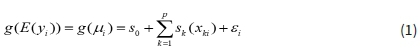
where g is a link function that links the expected value to the predictor variables, μ. is the expectation of the response variabley,, s₀is the overall means of the response, s_k{x_h) is the smooth function of i^th value of covariate k,p is the total number of covariates, and ε. is the i^th residual which is assumed to be normally distributed: . The smooth function was used to minimize the penalized residual sum of squares (shown in equation 2):

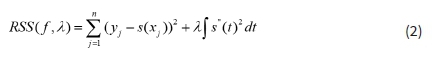
The term evaluates the closeness to the data and penalizes curvature in the function. λ is a fixed smoothing parameter. The increase of the value of λ provides a smoother function. The choice of this parameter becomes critical given the flexibility of the GAM model and the risk of over-fitting. Generalized Cross Validation (GCV) is the most used method to fix the smoothing parameter λ. In this paper, the main purpose is to find the combination of explanatory variables which can describe a high degree of the pollutant concentration variability (R²) in Tunis. In order to analyze the seasonality of O₃ and PM₁₀ concentrations that exist in this data, we started by fitting a preliminary base model with time variables only (equation 3):

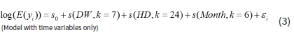
The variable day of the week (DW) was used to account for weekly variations. Also, the predictor hour of the day (HD) was employed with values ranging from 1 to 24. This variable is meant to take care of diurnal variation that is not explained by the other variables. Additionally, since air pollution data are known to be seasonal, k which is the maximum number of knots for each smoother. The smoothing spline for HD had 24 knots and was employed to account for processes on time scales larger than one hour. The variable DW had 7 knots one for each day. Finally, the variable Month was employed with k = 6. Both residuals histograms and scatter plots confirmed the adequacy of this choice of k values (see the section "Assessment of the model performance").

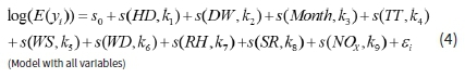
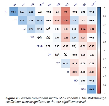
Tropospheric ozone O₃ and particulate matter PM₁₀ concentrations were modeled separately using the model given by (equation 4), with five meteorological variables, temperature (TT°), Relative Humidity (RH %), Solar Radiation (SR W.nr²), Wind Speed (WS m.s^-1),Wind Direction (WD degree from the north) applied via the GAM modeling function in the R environment for statistical computing inside the "mgcv" package (Wood, 2006). Traffic data and precipitation data were not available in the study areas. Therefore, three temporal variables and some traffic related air pollutant data were included to roughly account for traffic density and industrial emissions. Nitrogen oxides (NO_X μg.m^-3) was used as explanatory variables instead traffic flow data (Pont and Fontan, 2000) and to represent a source for secondary particle matter. The predictor variables are slightly correlated (Fig. 4). For example, the correlation between the wind speed and the solar radiation is 0.26, between the temperature and hour of the day, it is 0.2. A strong negative linear relationship was detected between relative humidity and temperature (-0.66) and between relative humidity and solar radiation (-0.6). Most other correlation coefficients are 0.50 or less in absolute values. Based on these moderate correlations, we do not expect any serious problems with confounding effects between predictor variables. In this study, the Variance Inflation Factor (VIF definition in Appendix A) was used to detect the multicollinearity of variables (Belusic, Herceg-Bulic and Bencetic Klaic, 2015) and the multicollinearity is considered very important when VIF values are higher than 10 (Graham, 2003). For all variables, VIF values were lower and ranged from 1.001 for the day of the week (DW) to 2.934 for the temperature. Thus, we assumed that all variables are not collinear, and a regression method could be applied. In order to select the final model, meteorological variables were added to the base model (equation 3) upon which Akaike's Information Criteria (AIC) was calculated. A variable remained in the final model if the fit yielded a lower AIC. Finally, the model for each pollutant can be written as:

 

 

 

The maximum number of knots for each smoother k must be chosen before the smoothing function is estimated. It controlled the smoothness of each function s_k(x_kj) in the final model. This particular parameter should be large enough so that the main process which governs concentrations values are included in the model. Many studies were employed forward validation which is a special form of cross-validation and is considered as the easiest method to choose optimal knots (Aldrin and Haff, 2005; Belusic, Herceg-Bulic and Bencetic Klaic, 2015). So, in this work, forward validation for each pollutant was based on hourly predictions of concentrations for Tunis, one day in advance. For each day and for the maximum number of knots, the model was re-estimated using the data up to the day before. Then, the hourly log PM₁₀ and log O₃ concentrations for the next day are predicted. The prediction is compared to the logarithm of the observed value and the hourly prediction errors calculated. For each day and for each of the two pollutants, this procedure was repeated. The root mean square (RMSE) of the prediction was finally calculated (RMSE definition in Appendix A). The minimum RMSE for each pollutant corresponded to k = 15 for (Temperature (TT°), nitrogen oxides (NO_X μg.m^-3)) and k = 10 for (relative humidity (RH %), solar radiation (SR W.m^-2)). The value of k = 8 was large enough only for wind variables.

 

Results and discussion

Based on the data described in Section "Site description and sample collection", the additive model with all variables was estimated for the two pollution variables PM₁₀ and O₃ recorded at three different stations in Tunis.

The first two columns of Table 2 show the explained variation (squared correlation coefficients R2) for the entire model (equation 4). The second part of the table presents the explained variation for meteorological variables only (R2m.v) which measured the aggregate impacts of local meteorology on each pollutant. R2m.v corresponds to the explained variation of a new model given by the difference of the models with only time variables and with all variables. The highest values of R2 were obtained for O₃ at Bab Aliwa station. We found that the explained variance for the entire model is between 0.56 and 0.85, indicating that the models explain most of the variation in pollutant concentrations, but a considerable amount of variation is still unexplained. The aggregate impact of meteorological variables was measured between 0.21 and 0.42.

Ozone

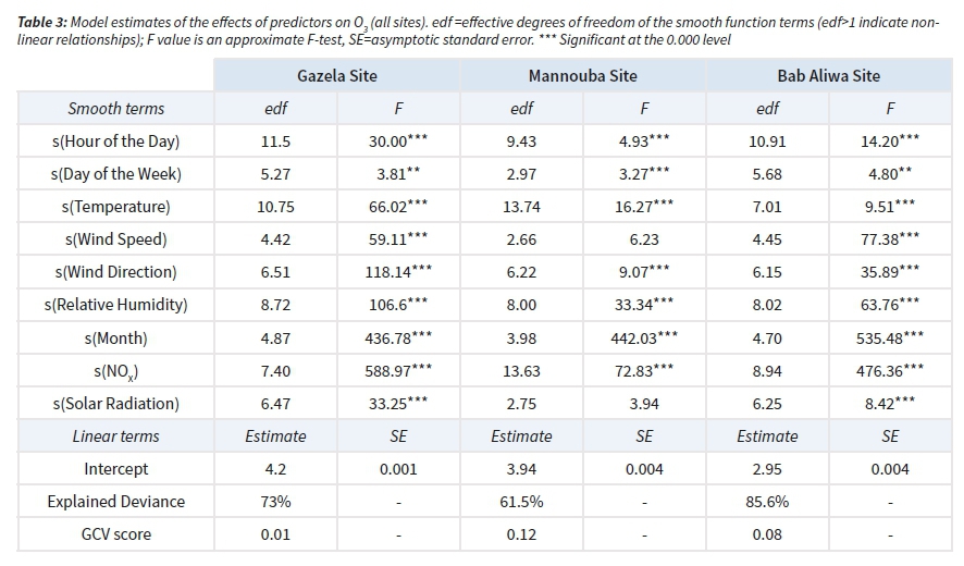
Tropospheric ozone is considered a secondary pollutant which is formed by photochemical reactions involving the oxides of nitrogen NO and NO₂ (summed as NO_X), hydrocarbons and sunlight, particularly ultraviolet light. In urban areas, high ozone levels are observed during warm summer months when the temperature is high and the wind velocity is low. In Tunis, we found that the final model explained 85% (site of Bab Aliwa) of the variance of log-transformed O₃ concentrations (Table 2). The aggregate impact of meteorological variables explained 41% of the variance in O₃ for the same site (Bab Aliwa). The estimated effects of meteorological and temporal variables on O₃ are shown in Fig. 5 (a), (b) and (c) for three stations in Tunis. Most meteorological, traffic and temporal factors were statistically significant in a highly non-linear way.

The influence of local meteorology on O₃

Temperature effect

For all three measurement stations, temperature (TT) was an important meteorological variable for O₃. The effect of temperature on O₃ is similar at Gazela and Bab Aliwa sites. A positive effect is seen for temperatures ranging between 5°C-20°C across only these two sites. A negative effect is noted for temperatures ranging between 20°C and 40°C for all three sites. So, if temperature increases, ozone concentrations are seen to decrease. This disagrees with common understanding of this relationship (Cheng et al., 2007; Polinsky and Shavell, 2010; Pearce et al., 2011; Ma et al., 2020), but can due to correlations of temperature with other variables like wind direction. The formation and concentration of ground level O₃ depends on the concentrations of NO_X and VOCs, and the ratio of NO_X and VOCs. Ozone levels do not always increase with increases in temperature, such as when the ratio of VOCs to NO_X is low. As study area was surrounded by reliefs, the speeds of surface winds are low. It may be more thermal breezes than synoptic-scale winds (Melki, 2007). The high frequency of thermal breezes and calm periods may indicate stable atmospheric conditions and thus O₃ concentrations are higher during such episodes.

Wind effect

The curves in the center of Fig. 5 (a), (b) and (c) show the results obtained regarding the impact of wind direction. The estimated response for the wind direction is different for the various locations. This is as normal, since the effect of wind direction is strongly correlated on the emission locations. A non-linear relationship is observed for all stations: edf=6.51, edf=6.22 and edf=6.15 at Gazela, Mannouba and Bab Aliwa, respectively (Table 3). At the first site, O₃ exhibits maximum concentration for E-NE wind (70°-100°) and minimum concentration at around 200°. However, by examining the wind speed-direction frequencies graph of this site (Fig. 6), there is a very remarkable effect of this variable on ozone concentration. A possible explanation is the location of this measuring site which is subject to northern European pollution (i.e. O₃ is transported from Italy to Tunis). While crossing the city towards Mannouba site, the effect of wind decreases. In this station, O₃ shows secondary maxima for S-W wind (250°). The wind direction at the Bab Aliwa site seems to have a different effect on O₃ concentration. Wind direction has a positive effect on O₃ concentration for directions between 100° and 250°. This is probably associated with the cemetery effect which promotes ozone's transport. A light minimum is then observed at 270°. The effect of road traffic can explain this. In this study, increasing wind speed was found to correspond to increasing O₃ concentrations. This tendency is particularly marked for the Bab Aliwa station (Figure 5c). This agrees with previous findings of Melki, (2007). At the Gazela site, the effect of this variable is very local, so, difficult to explain. It may be possible to understand this effect on a scale larger than a city.

Solar radiation and relative humidity effects

Solar radiation had a non-linear association: edf=6.47, edf=2.75 and edf= 6.25 at Gazela, Mannouba and Bab Aliwa, respectively, (Table 3) with O₃ concentrations. These results are very clear, higher solar radiation corresponds to higher concentrations of O₃. This positive effect was found to be strongest after values surpassed 400 W.m^-2 (Gazela and Bab Aliwa station). This relationship is consistent with the literature (Pearce et al., 2011) as radiation plays a significant role in photochemistry of ozone production (Dawson, Adams and Pandis, 2007). The nature of response of O₃ to the RH showed a 10% under low RH, and then exhibited a modest negative relationship where high levels resulted in a regional decrease of up to 10% for Gazela and Mannouba, and 5% for Bab Aliwa. So, the curves go downward for increasing humidity. Generally, the results obtained in this analysis of meteorological parameters were expected, i.e. that higher ozone concentrations were associated with high temperature, low relative humidity and prolonged sunshine (Lacour et al., 2006). In this coastal region of the northern Mediterranean, at night the relative humidity of the air is important (96% on average), combined with a decline in temperature (18°C on average). This conjunction will reduce O₃ concentrations.

The impact of time and traffic variables on O₃

The upper left panel of Fig. 5 (a), (b) and (c) show how the concentrations of O₃ varies as the hour of the day (HD) changes. Each curve corresponds to one of the measurements stations. Since this variable describes the diurnal variation of O₃ in three locations, different curves are observed. The diurnal variation for Mannouba and Bab Aliwa sites shows a similar pattern with O₃ concentrations reaching the peak at around 9:00 at the Mannouba site and at around 14:00 at the Bab Aliwa site. The increase in O₃ concentrations during day time is due to the increase in solar radiation, which powers the photochemical reactions and consequently O₃ concentration (Khoder, 2009). The hour's period of negative effect is presumably due to high emissions of NO_X caused by the intensity of traffic. Monks et al. (2015) highlighted the non-linearity of the O₃-VOC-NO_X system. VOC-limited refers to the fact that the production of O₃ is limited by the input of VOC. Indeed, high NO_X lead to lower O₃ because O₃ directly react with NO. The local production of ozone is less reduced because the NO_X react with hydroxyl radical species formed in the atmosphere. When these hydroxyl radicals do not react with NO_X (example: low emission of NO_X), they contribute to the VOC degradation and the ozone production. Unlike other sites, Gazela is considered a residential site which is characterized by the domination of NO_X emissions (at this site, VOCs are only due to traffic, and not as much emitted as by factories like the other sites). In fact, a minimum of O₃ concentration is observed at around 8:00 and a maximum at around 19:00 when traffic is an important source of emissions and the vertical mixing is reduced. Influenced by transport of O₃ from other regions and local NO_X concentrations at night, the increase of the surface O₃ concentration during the night time was larger than that during the daytime (Lei and Wang, 2014). Day of the week at Gazela and Mannouba (Table 3) was found to have little influence on ozone, (F=3.81, F=3.27. respectively). For Monday to Wednesday the ozone concentrations remain more or less unchanged (Figure 5). The rise in ozone concentrations is observed on Thursday and Friday but is followed by a drop as of Saturday. This continues on Sunday when the levels of ozone then join those on Monday. This result was also found by Pont and Fontan (2000) for five large French cities: This study does not show any significant variation in ozone concentrations between weekend and week except for the strongest values where a 40% reduction in precursors would lead to a 20% increase in ozone. The weekend effect would be reversed. Due to constant of road traffic during all the days of the week in Bab Aliwa, no effect of the variable DW was observed. NO_X also has a non-linear association with O₃ concentration, with edf=7.40 and edf=8.94 at Gazela and Bab Aliwa, respectively (Table 3). Increased NO_X for these two sites was found to have a negative effect on O₃. This finding is in agreement with other work since the chemical coupling of O₃ and NO_X make levels of O₃ inextricably linked: Ozone production is dependent on the state of NO_X, as NO₂ and NO increase the production and dissociation of O₃, respectively. Consequently, an increased NO/NO₂ ratio reduces the ozone concentration (Melkonyan and Kuttler, 2012). Analysis the results of Mannouba station reveals a different NO_X effect, when the NO_X concentrations is over 200 ppb, an increase of NO_X concentrations leads to a lower decrease of O₃ concentrations than at the other stations. An increase in O₃ concentrations is seen above 280 ppb of NO_X concentrations. This is presumably due to the location of this station, which includes small forests in the west and chemical plants in the south which promote VOCs emissions, then the increase of both O₃ and NO_X concentrations. A positive effect is detected for the variable Month on O₃ concentration in warm months (spring and summer). In this period, there is an increase in temperatures and in the intensity of solar radiation. These meteorological conditions promote the mixing process of pollutants and O₃ formation. The ozone evolution is controlled not only by the influence of climate but also by the movement of pollutants. In fact, the same result was found in two regions: Spain and Italy which belong to the Mediterranean climate (Domínguez-López et al., 2014; Myriokefalitakis et al., 2016).

PM10

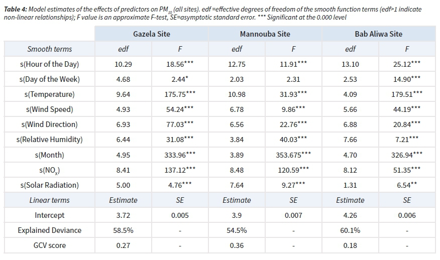
The impact of traffic and site location on PM₁₀ Atmospheric PM₁₀ are multicomponent aerosols. They originate from a variety of mobile, stationary and other natural sources, and are also formed in the atmosphere through chemical and physical processes. SO₂ (mainly issued from industrial sector) and NO_X (mainly issued from transport sector) are two precursors of secondary particulate matter (Harrison, Jones and Lawrence, 2004). Their chemical and physical compositions vary widely. Many studies showed that the PM₁₀ yearly, daily and hourly average concentration exceeds the Tunisian and the European standard limits at all the sampling stations (Bouchlaghem et al., 2009). A significant proportion of PM₁₀ in Tunis has many sources like sea salt, mineral dust (Calzolai et al., 2015). In the Mediterranean Tunisian regions, the average seasonal evolution of PM₁₀ is characterized by a winter maximum (November and December) (Bouchlaghem and Nsom, 2012). On the other hand, ozone concentration reaches its maximum values during summer period under the great photochemical activity and the effect of land-sea breeze. This difference has been highlighted in many studies and has been explained by the formation of PM₁₀ as a complex mixture of many chemical species. Indeed, both the proximity to traffic sources and the different types of air mass scenarios make PM₁₀ formation rather complex and associated with geographic, temporal and meteorological conditions. In Tunis, we found that the final model explained between 56% and 59% of the variance of log-transformed PM₁₀. The highest value of R² was found at Bab Aliwa station and the aggregate impact of meteorological variables accounting for 29%. The estimated effects of independent variables of the model are shown in Fig. 7 (a), (b) and (c) for three stations in Tunis. The model shows how the association of PM₁₀ concentrations varies with the levels of other variables. The association between NO_X concentrations and PM₁₀ concentrations was non-linear with edf=8.41,edf=8.48 and edf=8.12 at Gazela, Mannouba and Bab Aliwa respectively (Table 4) and is characterized by a general positive effect. It is reasonable and also found in Munir et al. (2013). Actually both NO_X and PM₁₀ are largely issued from road traffic. The curve for Bab Aliwa is the one going farthest to the right meaning that it is the location where the highest number of vehicles was observed. This might be logically explained by the fact that in this location, we found the biggest bus station and the most popular cemetery in the country. SO₂ and NO_X are the two sources of secondary particulate matter and have mostly a positive effect on PM₁₀ (Harrison, Jones and Lawrence, 2004). NO_X concentration in Gazela station may be affected by Tunis airport located in the South east of the station.

 

The influence of local meteorology on PM₁₀

A non-linear association was observed between PM₁₀ and wind speed. This variable has a positive effect on PM₁₀ concentration from 4 m.s^-1 to 8 m.s^-1 at Gazela site. The curves for Mannouba and Bab Aliwa (Fig. 7 (b) and Fig. 7 (c)) reached the peak at 5 m.s^-1 then decrease. The same wind behavior was observed in three sites and was found in Belusic, Herceg-Bulic and Bencetic Klaic (2015): For large wind speeds, PM₁₀ concentration decrease. This result was as expected as low wind and stable atmospheric conditions support higher concentrations of PM₁₀. We note however that the decrease in PM₁₀ levels at higher winds observed in the present study is in contrast to the result found in Makkah by Munir et al., (2013) and in Maribor by Lesnik, Mongus and Jesenko (2019). Wind direction had variable association with PM₁₀: edf=6.88 at Bab Aliwa site (Table 4). Several curves were observed for different sites. In the first station, Gazela, (center of Fig. 7 (a)), PM₁₀ exhibit a first maximum concentration for wind direction around 170°. This can be explained by localized effect of the road. The secondary maximum is observed around 320°, clearly reflecting the effect the small factory situated north of the study area. As Bab Aliwa is based next to taxi and bus stations, this particular measuring site is subject to PM₁₀ transport by southeast winds. For relative humidity, the results are very clear especially for Gazela and Mannouba sites, which find that high humidity was associated to low PM₁₀ concentration. So, the curves go downward for humidity better than 80%.This agrees with previous findings of Aldrin and Haff (2005) and Belusic, Herceg-Bulic and Bencetic Klaic (2015). Particles are then removed from contaminated surface air by wet deposition in precipitation added to dry deposition (Giri, Murthy and Adhikary, 2008). The estimate curves of temperature have the same slope for the various locations. Temperature was named as the most significant meteorological variable for Bab Aliwa (F=179.51, p-value <0.001) and Gazela (F=175.75, p-value <0.001) sites. Interpretation of the curves (lower left of Fig. 7 (a), (b) and (c)) can be expressed as follows: increasing temperature corresponds with increasing PM₁₀ with a notable positive effect for temperature above 20°C. It's important to note that this finding agrees the result from PM₁₀ studies (Bouchlaghem and Nsom, 2012). However, the positive relationship between temperature and PM₁₀ is probably explained by the dust layer created over three sites especially during peak hours.

The impact of time variables on PM₁₀

The time variable hour of the day (HD) has a non-linear association with PM₁₀ concentration. It was mainly used to account the effect of traffic. At the study stations, PM₁₀ concentration fall to a minimum between 7:00-8:00 and increase until 10:00, this corresponds to the morning peak traffic flow. In Bab Aliwa site, an evening peak traffic flow was noted at around 21:00. This second peak is probably due to people's daily commuting between the capital and the suburbs. Curves of partial effect of the variable Month pointed out that in all measuring sites, PM₁₀ is characterized by a winter maximum (December-January-February). This result is consistent with the data of Bouchlaghem and Nsom (2012), who found a winter PM₁₀ peak in five different stations (traffic, industrial and residential) in Tunisia. This is presumably due to the influence of low mixing in the atmosphere and the advection of Saharan plumes. We note the absence of the second peak observed during the summer in the previous works (Bouchlaghem and Nsom, 2012). The slight effect of Saharan dust can be explained by the temporal difference between the South and the North of Tunisia and the geographical locations of the monitoring stations far from the southwest origin of the Saharan event. Since the Mannouba station is placed close to agriculture fields, plowing during the autumn season (September-October) promotes increasing PM₁₀ concentrations.

 

Assessment of the model performance

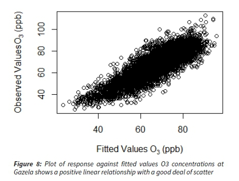
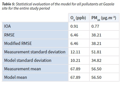
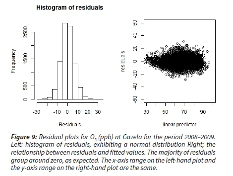
Various metrics (RMSE, modified RMSE, measurement standard deviation, model standard deviation and IOA (see Appendix A)) were used to assess the model performance. This statistical evaluation of the model on the original scale is presented in Table 5 is for all variables at Gazela site; other pollutants and measuring site data are not shown here as the results are similar to these. The first criterion for model evaluation was checked and both RMSE and Modified RMSE are less than measurement standard deviation. In addition, the index of agreement is 0.91 and 0.77 for O₃ and PM₁₀, respectively, which corresponds to a good compromise between modeled and measured values. Fig. 8 shows the relationship between the response and fitted values of O₃ concentration at Gazela site. PM₁₀ and other measuring site data are not shown as they are similar to those presented in this figure. This figure shows a positive linear relationship with a good deal of scattering. Residual plots are also used to characterize model efficacy. Fig. 9 clearly shows that the majority of residuals group around zero, as expected. The right-hand scatter plot which describes the relationship between residuals and fitted values suggest that variance is approximately constant as the mean increases. The left-hand plot, the residual histogram, exhibits a normal distribution for O₃ at Gazela.

 

 

 

 

 

 

Conclusions

The objective of this work was to estimate the relationship between each of two pollution variables, namely concentrations of PM₁₀ and tropospheric ozone O₃ and NO_X concentrations (taking as a proxy of traffic) as well as a set of meteorological variables for the urban area of Tunis. To achieve this objective, a statistical methodology is used based on the Generalized Additive Model (GAM). We have shown that the GAM can model the non-linear effect of the covariates. The model is additive on the log scale and the estimates were made on hourly data collected during two years at three different locations in Tunis. The model provides a reasonably good fit in terms of the explained variance. For all stations, O₃ was easier to model (i.e. with more explanatory power and higher values of R2). The most significant important variables for O₃ are NO_X, wind direction and relative humidity. The impact of temperature and NO_X is the strongest for PM₁₀, followed by relative humidity and wind variables. The time variables (hour of the day, day of the week and month) appear to have a particular impact on air quality. In this study, the variable Month plays a significant role in the characterization of the study area as a function of time. In fact, we note the seasonal behavior of O₃ and PM₁₀ pollutants, with the highest concentrations in summer and winter, respectively. These results allow a first and fast analysis of the air pollution due to O₃ and PM₁₀ in 3 locations in Tunis. It emphasizes the critical role of the local conditions on the air pollution, and especially the emissions and the weather as two main drivers of urban air pollution. Our findings suggest focusing on model improvement as future work. The addition of precipitation and traffic density (number of vehicles) variables could help to improve the model assessment. So, it is necessary to take into account all the sources of emissions exhaustively. In summary, the use of GAM in combination with partial residual plots offered an effective way to outline the relationships between temporal, meteorological and traffic variables and air pollution. Although our study did not detail chemical and physical aspects of air pollution, the results produced were reasonable and comparable to other studies. Furthermore, the results may be considered as relevant because research work on air pollution is insufficient in Tunisia. To this end, after quantifying the influence of all used variables, we plan to use GAM and GAMM (Hastie and Tibshirani, 1990; Wood, 2006) models to forecast pollutant concentrations.

 

References

Aldrin, M. and Haff, I.H. (2005) 'Generalised additive modelling of air pollution, traffic volume and meteorology', Atmospheric Environment, vol. 39, pp. 2145-2155. https://doi.org/10.1016/j.atmosenv.2004.12.020        [ Links ]

Ayari, S., Nouira, K. and Trabelsi, A. (2012) 'A Hybrid ARIMA and Artificial Neural Networks Model to Forecast Air Quality in Urban Areas: Case of Tunisia', Advanced Materials Research, vol. 518523, pp. 2969-2979. https://doi.org/10.4028/www.scientific.net/AMR.518-523.2969        [ Links ]

Belhout, D., Rabah, K., Helder, R. and Ana, M. (2018) 'Air quality assessment in Algiers city', Air Quality, Atmosphere & Health, vol. 11, October, pp. 1-10. https://doi.org/10.1007/s11869-018-0589-x        [ Links ]

Belušić,, A., Herceg-Bulić, I. and Bencetić Klaić, (2015) 'Using a generalized additive model to quantify the influence of local meteorology on air quality in Zagreb', Geofizika, vol. 32, pp. 47-77.https://doi.org/10.15233/gfz.2015.32.5        [ Links ]

Bouchlaghem, K. and Nsom, B. (2012) 'Effect of Atmospheric Pollutants on the Air Quality in Tunisia', The Scientific World Journal. https://doi.org/10.1100/2012/863528        [ Links ]

Bouchlaghem, K., Nsom, B., Latrache, N. and Hadj Kacem, H. (2009) 'Impact of Saharan dust on PM₁₀ concentration in the Mediterranean Tunisian coasts', Atmospheric Research, vol. 92, pp. 531-539. https://doi.org/10.1016/jJ.atmosres.2009.02.009        [ Links ]

Bourdrel, T., Bind, M.A., Béjot, Y., Morel, and Argacha, J.F. (2017) 'Effets cardiovasculaires de la pollution de l'air', Archives of Cardiovascular Diseases, vol. 110, pp. 634-642.https://doi.org/10.1016/j.acvd.2017.05.003        [ Links ]

Calzolai, G., Nava, S., Lucarelli, F., Chiari, M., Giannoni, M., Becagli, S., Traversi, R., Marconi, M., Frosini, D., Severi, M., Udisti, R., Di Sarra, A., Pace, G., Meloni, D., Bommarito, C., Monteleone, F., Anello, F. and Sferlazzo, D.M. (2015) 'Characterization of PM₁₀ sources in the central Mediterranean', Atmospheric Chemistry and Physics, vol. 15, pp. 13939-13955. https://doi.org/10.5194/acp-15-13939-2015        [ Links ]

Cheng, C.S., Campbell, M., Li, Q., Li, G., Auld, H., Day, N., Pengelly, D., Gingrich, S. and Yap, D. (2007) 'A synoptic climatological approach to assess climatic impact on air quality in south-central Canada. Part I: Historical analysis', Water, Air, and Soil Pollution, vol. 182, pp. 131-148.https://doi.org/10.1007/s11270-006-9327-3        [ Links ]

Chirmata, A., Leghrib, R. and Ichou, I. (2017) 'Implementation of the Air Quality Monitoring Network at Agadir City in Morocco', Journal of Environmental Protection, vol. 08, pp. 540-567.https://doi.org/10.4236/jep.2017.84037        [ Links ]

Dawson, J.P., Adams, P.J. and Pandis, S.N. (2007) 'Sensitivity of ozone to summertime climate in the eastern USA: A modeling case study', Atmospheric Environment, vol. 41, pp. 1494-1511. https://doi.org/10.1016/j.atmosenv.2006.10.033        [ Links ]

Dehghan, A., Khanjani, N., Bahrampour, A., Goudarz, G. and Yunesian, M. (2018) 'The relation between air pollution and respiratory deaths in Tehran, Iran- using generalized additive models', BMC Pulmonary Medicine, vol. 18, no. 1, p. 49. https://doi.org/10.1186/s12890-018-0613-9        [ Links ]

Directive, E. (2008) Directive 2008/50/EC of the European Parliament and of the Council, [Online], Available: http://www.era-comm.eu/Cooperation_national_judges_environmental_ law/module_4/02.pdf.         [ Links ]

Domínguez-López, D., Adame, J.A., Hernández-Ceballos, M.A., Vaca, F., De la Morena, B.A. and Bolívar, J.P. (2014) 'Spatial and temporal variation of surface ozone, NO and NO₂ at urban, suburban, rural and industrial sites in the southwest of the Iberian Peninsula', Environ MonitAssess. https://doi.org/10.1007/s10661-014-3783-9        [ Links ]

Giri, D., Murthy, K. and Adhikary, P.R. (2008) 'The Influence of Meteorological Conditions on PM₁₀ Concentrations in Kathmandu Valley', Int. J. Environ. Res, vol. 2, pp. 49-60. https://doi.org/10.22059/IJER.2010.175        [ Links ]

Graham, M.H. (2003) ''Statistical Confronting Multicollinearity in Ecological'', Ecological Society of America, vol. 84, pp. 2809-2815. https://doi.org/10.1890/02-3114        [ Links ]

Harrison, R.M., Jones, A.M. and Lawrence, R.G. (2004) 'Major component composition of PM₁₀ and PM₂₅from roadside and urban background sites', Atmospheric Environment, vol. 38, pp. 4531-4538. https://doi.org/10.1016/j.atmosenv.2004.05.022        [ Links ]

Hastie, T.J. and Tibshirani, R. (1990) 'Generalized additive models', Statistical Science, vol. 1, pp. 297-318. https://doi.org/10.1214/ss/1177013604        [ Links ]

He, S., Mazumdar, S. and Arena, V.C. (2005) 'A comparative study of the use of GAM and GLM in air pollution research', Environmetrics, vol. 17, pp. 81-93. https://doi.org/10.1002/ env.751        [ Links ]

INS (2014) Tunisie en chiffres 2013 - 2014, [Online], Available: http://www.ins.tn/publication/tunisie-en-chiffres-2013-2014.         [ Links ]

Karaca, F., Nikov, A. and Alagha, O. (2006) 'AirPolTool - A WEB-BASED TOOL FOR ISTANBUL Air Pollution Forecasting And Control', Int. J. Environment and Pollution, vol. 28, pp. 3-4.https://doi.org/10.1504/IJEP.2006.011214        [ Links ]

Khoder, M.I. (2009) 'Diurnal, seasonal and weekdays-weekends variations of ground level ozone concentrations in an urban area in greater Cairo', Environmental Monitoring and Assessment, vol. 149, pp. 349-362. https://doi.org/10.1007/s10661-008-0208-7        [ Links ]

Lacour, S.A., De Monte, M., Diot, P., Brocca, J., Veron, N., Colin, P. and Leblond, V. (2006) 'Relationship between ozone and temperature during the 2003 heat wave in France: Consequences for health data analysis', BMC Public Health. https://doi.org/10.1186/1471-2458-6-261        [ Links ]

Lei, H. and Wang, J.X.L. (2014) 'Sensitivities of NO_X transformation and the effects on surface ozone and nitrate', Atmospheric Chemistry and Physics, vol. 14, pp. 1385-1396. https://doi.org/10.5194/acp-14-1385-2014        [ Links ]

Lesnik, U., Mongus, D. and Jesenko, D. (2019) 'Predictive analytics of PM₁₀ concentration levels using detailed traffic data', Transportation Research Part D, pp. 131-141. https://doi.org/10.1016/j.trd.2018.11.015        [ Links ]

Ma, Y., Ma, B., Jiao, H., Zhang, Y., Xin, J. and Yu, Z. (2020) 'An analysis of the effects of weather and air pollution on tropospheric ozone using a generalized additive model in Western China: Lanzhou, Gansu', Atmospheric Environment, vol. 224, March, p. 117342. https://doi.org/10.1016/j.atmosenv.2020.117342        [ Links ]

Melki, T. (2007) ''Inversions Thermiques Et Concentrations De Polluants Atmospheriques Dans La Basse Troposphere De Tunis', Climatologie, vol. 4. https://doi.org/10.4267/climatologie.773        [ Links ]

Melkonyan, A. and Kuttler, W. (2012) 'Long-term analysis of NO, NO₂ and O₃ concentrations in North Rhine-Westphalia, Germany', Atmospheric Environment, vol. 60, pp. 316-326. https://doi.org/10.1016/j.atmosenv.2012.06.048        [ Links ]

Monks, P.S., Archibald, A.T., Colette, A., Cooper, O., Coyle, M., Derwent, R., Fowler, D., Granier, C., Law, K.S., Mills, G.E., Stevenson, D.S., Tarasova, O., Thouret, V., von Schneidemesser, E., Sommariva, R., Wild, O. and Williams, M.L. (2015) 'Tropospheric ozone and its precursors from the urban to the global scale from air quality to short-lived climate forcer', Atmospheric Chemistry and Physics, vol. 15, no. 15, pp. 8889-8973. https://doi.org/10.5194/acp-15-8889-2015        [ Links ]

Munir, S., Habeebullah, T.M., Seroji, A.R., Morsy, E.A., Mohammed, A.M.F., Saud, W.A., Abdou, A.E.A. and Awad, A.H. (2013) 'Modeling particulate matter concentrations in Makkah, applying a statistical modeling approach', Aerosol and Air Quality Research, vol. 13, pp. 901-910. https://doi.org/10.4209/aaqr.2012.11.0314        [ Links ]

Myriokefalitakis, S., Daskalakis, N., Fanourgakis, G.S., Voulgarakis, A., Krol, M.C., Aan de Brugh, J.M.J. and Kanakidou, M. (2016) 'Ozone and carbon monoxide budgets over the Eastern Mediterranean', Science of the Total Environment, vol. 563-564, pp. 40-52. https://doi.org/10.1016/j.scitotenv.2016.04.061        [ Links ]

Pearce, J.L., Beringer, J., Nicholls, N., Hyndman, R.J. and Tapper, N.J. (2011) 'Quantifying the influence of local meteorology on air quality using generalized additive models', Atmospheric Environment, vol. 45, pp. 1328-1336. https://doi.org/10.1016/j.atmosenv.2010.11.051        [ Links ]

Polinsky, A.M. and Shavell, S. (2010) 'The uneasy case for product liability', Harvard Law Review, vol. 123, pp. 1437-1492.         [ Links ]

Pont, V. and Fontan, J. (2000) 'Local and regional contributions to photochemical atmospheric pollution in southern France', Atmospheric Environment, vol. 34, pp. 5209-5223. https://doi.org/10.1016/S1352-2310(00)00353-8        [ Links ]

Rahal, F., Benharrats, N., Blond, N., Ponche, J.-L. and Clappier, A. (2014) 'Modelling of air pollution in the area of Algiers City, Algeria', International Journal of Environment and Pollution, vol.54, pp. 32-58. https://doi.org/10.1504/IJEP.2014.064049        [ Links ]

Ravindra, K., Rattan, P., Mor, S. and Nath Aggarwal, A. (2019) 'Generalized additive models: Building evidence of air pollution, climate change and human health', Environment International, vol. 132, no. ISSN 0160-4120, Novembre, p. 104987. https://doi.org/10.1016/j.envint.2019.104987        [ Links ]

Saffarini, G. and Odat, S. (2008) 'Time Series Analysis of Air Pollution in Al-Hashimeya Town Zarqa, Jordan', Jordan Journal of Eart and Environmental Sciences, vol. 1, pp. 63-72.         [ Links ]

Schlink, U., Dorling, S., Pelikan, E., Nunnari, G., Cawley, G., Junninen, , Greig, A., Foxall, R., Eben, K., Chatterton, T., Vondracek, J., Richter, M., Dostal, M., Bertucco, L., Kolehmainen, Kolehmainen, M. and Doyle, M. (2003) 'A rigorous inter-comparison of ground-level ozone predictions', Atmospheric Environment, vol. 37, pp. 3237-3253. https://doi.org/10.1016/S1352-2310(03)00330-3        [ Links ]

Sinharay, R., Gong, J., Barratt, B., Ohman-Strickland, P., Ernst, S., Kelly, F., Zhang, J.(., Collins, P., Cullinan, P. and Chung, K.F. (2017) 'Respiratory and cardiovascular responses to walking down a traffic-polluted road compared with walking in a traffic-free area in participants aged 60 years and older with chronic lung or heart disease and age-matched healthy controls: a randomised, crosso', The Lancet, vol. 391, pp. 339-349. https://doi.org/10.1016/S0140-6736(17)32643-0        [ Links ]

Taheri Shahraiyni, H., Sodoudi, S., Kerschbaumer, A. and Cubasch, (2015) 'The development of a dense urban air pollution monitoring network', Atmospheric Pollution Research, vol. 6, pp. 904-915. https://doi.org/10.5094/APR.2015.100        [ Links ]

WHO (2006) 'WHO air quality guidelines for particulate matter, ozone, nitrogen dioxide and sulfur dioxide: global update 2005, summary of risk assessment. The publisher in WHO in Geneva.         [ Links ]

WHO (2016) ''World Health Statistics - Monitoring Health for the SDGs', pp. 1-121.         [ Links ]

Wood, S. (2006) 'Generalized additive models: an introduction with R', Biometrics, vol. 62, p. 392. https://doi.org/10.1201/9781420010404        [ Links ]

Yang, J., Zhang, , Chen, Y., Ma, L., Yadikaer, R., Lu, Y., Lou, P., Pu, , Xiang, R. and Rui, B. (2020) 'A study on the relationship between air pollution and pulmonary tuberculosis based on the general additive model in Wulumuqi, China', International Journal of Infectious Diseases, vol. 96, pp. 42-47. https://doi.org/10.1016/_j.ijid.2020.03.032        [ Links ]

 

 

Received: 8 October 2020
Reviewed: 23 November 2020
Accepted: 10 September 2021

 

 

Appendix A

edf: The effective degrees of freedom (edf) estimated from generalized additive models were used as a proxy for the degree of non-linearity in stressor-response relationships. An edf of 1 is equivalent to a linear relationship, an edf > 1 and < 2 is a weakly non-linear relationship, and an edf > 2 indicates a highly nonlinear relationship.

GCV: generalized cross validation score can be taken as an estimate of the mean square prediction error based on a leave-one-out cross validation estimation process. We estimate the model for all observations except i, then note the squared residual predicting observation i from the model. Then we do this for all observations. GCV criteria is numerically stable and efficient, but its computation become extensive especially when several smoothing parameters have to be estimated.

F-statistic: An F statistic is a value you get when you run an ANOVA test or a regression analysis to find out if the means between two populations are significantly different. In regression case, the F value is the result of a test where the null hypothesis is that all of the regression coefficients are equal to zero. In other words, the model has no predictive capability. Basically, the f-test compares your model with zero predictor variables (the intercept only model), and decides whether your added coefficients improved the model.

Asymptotic Standard Error: Asymptotic standard error is an approximation to the standard error, based upon some mathematical simplification. In regression analysis, the term "standard error" refers either to the square root of the reduced chi-squared statistic, or the standard error for a particular regression coefficient (as used in, say, confidence intervals).

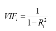
VIF: Variance Inflation Factor detects multicollinearity in regression analysis. For an independent variable X., it can be calculated by the formula below using R-squared values:

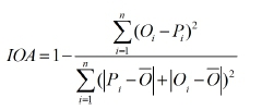
IOA: Index of Agreement is a standardized measure of the degree of model prediction error which varies between 0 and 1. IOA=1 represents full agreement and IOA=0 indicates no agreement at all.

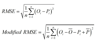
RMSE: The Root Mean Square Error is used to measure the difference between values predicted and values observed.