RESEARCH ARTICLE

 

Chemical characterization of fine particulate matter, source apportionment and long-range transport clusters in Thohoyandou, South Africa

 

 

Rirhandzu J. Novela^I; Wilson M. Gitari^{I, *}; Hector Chikoore^II; Peter Molnar^III; Rabelani Mudzielwana^I; Janine Wichmann^IV

^IEnvironmental Remediation and Nano Science Research Group, University of Venda, Private bag X5050, Thohoyandou, 0950 South Africa.
^IIUnit for Environmental Sciences and Management, North-West University, 1174 Hendrick Van Eck Boulevard, Vanderbijlpark, South Africa
^IIIOccupational and Environmental Medicine, Sahlgrenska University Hospital and University of Gothenburg, Medicinaregatan 16A, SE-40530, Sweden
^IVSchool of Health Systems and Public Health, University of Pretoria, 31 Bophelo Road, Pretoria, 0001 South Africa

 

 

---

ABSTRACT

This paper presents a chemical characterization of fine particulate matter (PM₂₅) in air masses passing through Thohoyandou and further determines their sources. PM₂₅ samples were collected and quantified using the gravimetric method. X-ray fluorescence, smoke stain reflectometer, optical transmissometer and scanning electron microscopy - energy dispersive X-Ray spectroscopy were used to determine the chemical and morphological composition of the particulate matter. The source apportionment was done using principal component analysis while the HYSPLIT model was used to depict the long-range transport clusters. The mean of concentrations of PM₂₅, soot, black carbon and UVPM were 10.9 ug/m³, 0.69x10^-5 m^-1, 1.22 μg/m³ and 1.40 μg/m³, respectively. A total of 24 elements were detected in the PM₂₅ with Pd, Sn, Sb, Mg, Al, and Si being the dominant elements. SEM-EDS have shown the presence of irregular, flat and spherical particles which is associated with crustal material and industrial emissions. Source apportionment analysis revealed six major sources of PM₂₅ in Thohoyandou namely, crustal materials, industrial emissions, vehicular emissions, urban emissions, fossil fuel combustion and fugitive-Pd. Air parcels that pass through Thohoyandou were clustered into four groupings. The major pathways were from the SW Indian Ocean, Atlantic Ocean, and inland trajectories. Clusters from the ocean are associated with low concentration, while inland clusters are associated with high concentration of PM₂₅. The PM₂₅ levels occasionally exceeded the daily WHO guideline (25 μg/m³) in Thohoyandou and the sources of PM₂₅ extend beyond the borders. This study recommends that further studies need to be carried out to assess the health impacts of PM₂₅ in Thohoyandou.

Keywords: PM₂₅ characterization; source apportionment; long range clusters; principal component analysis; backward trajectories.

---

 

 

Introduction

Ambient air pollution is a major environmental health issue globally due to several health implications associated with various air pollutants (Olaniyan et al., 2015). Of all air pollutants fine particulate matter (PM₂₅) is of major concern since it is linked to a number of health implications including premature death in adults with heart and lung disease, strokes, heart attacks, chronic respiratory disease such as bronchitis, aggravated asthma and premature deaths of children from acute lower respiratory infections such as pneumonia (CCAC, 2019). It is estimated that about 7 million people die prematurely every year as a result of exposure to PM₂₅ (WHO, 2014). The World Health Organization (WHO) has therefore set the daily guideline value of 25 μg/m³ for PM₂₅ concentrations in ambient air and further issued recommendations to countries to lower PM₂₅ levels in ambient air (WHO, 2016). In South Africa, the daily standard for PM₂₅ is set at 40 μg/m³ which is much higher compared to the WHO daily guideline.

Valsamakis (2015) conducted a study in Johannesburg, South Africa during winter and spring of 2013 and 2014 and recorded PM_2.5 concentrations at Petrus Molefe Eco Park ranging from 18.1-61.2 μg/m³ during spring and 62.9-126 μg/m³ during winter; 18.5-38.4μg/m³ during spring and 25.1-71.9 μg/m³ during winter at Thokoza Park. Biomass burning, vehicle emissions, industrial activity, and wind erosion of exposed areas were identified as major sources of particulate matter. Prior to that, Engelbrecht et al. (2002) had done source apportionment in Qalabotjha, South Africa and revealed that biomass burning is a major source of PM₂₅, accounting 13.8% of the PM₂₅ concentrations, and reported the daily range between 71 to 93 |g/m³. Biomass burning was also identified as a major contributor during the SAFARI 2000 dry season campaign through elemental analysis in Skukuza, South Africa (Petkova et al., 2013). In the Vaal Triangle and Johannesburg, biomass burning, and aged pollution-laden air have been responsible for 20-40% of inhalable particulates (DEA, 2009). The transportation industry is the second common source contributing to PM₂₅ concentrations through exhaust emissions, tire wear and dust resuspension. The growth of many cities without expanding or building new roads, together with increasing vehicle ownership result in a transportation system characterized by severe traffic congestion (Petkova et al., 2013) resulting in localized ambient air pollution. In Cape Town vehicle emissions have been identified as sources of brown haze (DEA, 2016). In Limpopo high emissions from vehicles are expected from national highways (N1 and N11) in Vhembe districts due to a high flow of vehicles as these roads connect South Africa to Zimbabwe and Botswana. On the South Africa environment outlook, DEA (2012) listed agricultural activities amongst sources that can be considered significant contributors to particulate emissions. Particulate emissions are derived from windblown dust, tillage and harvesting, dust entrainment due to heavy vehicles travelling (LEDET, 2016), fertilizer and chemical treatment, as well as the burning of residue crops and vegetation (DEA, 2012). The outcome of the huge dependence on coal in South Africa, is the high emission of particulate matter in coal fired power stations (DEA, 2016). These power stations have been identified as one of the leading sources of particulate matter in Limpopo (LEDET, 2016).

Air is a shared resource, not prone to any barriers circulating around the globe, whether clean or dirty. The geographical origin of the air mass can be traced through a combination of measurements and calculations using meteorological models (Wichmann et al., 2014). According to Tang et al., (2014) the contribution of long-range transport can be quantified using trajectory models such as the HYSPLIT model. The pathways that transport air masses away from and into South Africa is the Indian Ocean plume, the recirculation plume, the Atlantic ocean plume, the African plume and the Southern Ocean plume (DEA, 2009). Air masses from the south and central Atlantic are most likely to be free from industrial emissions. Air masses from the Indian Ocean are also relatively free of industrial pollutants, leaving the African transport plume, and carrying industrial pollutants from southern Africa (DEA, 2009). HYSPLIT trajectories have shown that Zambian copper belt emissions are transported over southern Africa (DEA, 2012), while in spring ambient air quality is likely to be affected by the transport of pollutants associated with biomass burning in the sub-equator (LEDET, 2016). Air pollution in South Africa also affects the neighboring countries (Swaziland, Lesotho, Mozambique, Zimbabwe and Botswana), with emissions from the Mpumalanga Highveld (Freiman and Piketh, 2002), while pollutants from Waterberg DM are anticipated to be transported and influence background concentrations in the North West Province (LEDET, 2016).

Although activities such as biomass burning, agricultural activities, construction and transportation are being carried out in Thohoyandou, no study has been conducted to quantify and characterize PM_2.5. These sources can be contributing to high PM_2.5 that are exceeding the standards and most likely to be detrimental to human health. Thus, this study is the first of its own kind in Limpopo. This study therefore aims at quantifying the PM₂₅ in Thohoyandou, Limpopo Province South Africa, the correlation between meteorological variables and PM_2.5 and further determines the chemical composition of quantified PM_2.5. Lastly the source apportionment of the contaminants as well as geographical origin of the air masses were determined using gravimetric method, principal component analysis and HYSPLIT model respectively.

 

Methods

Study area

Sampling of PM_2.5 was undertaken on the roof of the School of Environmental Sciences building, University of Venda. Figure 1 demonstrates Thohoyandou in Limpopo province, South Africa. Limpopo shares borders with three countries, Mozambique, Zimbabwe, and Botswana, and they can also contribute to PM_2.5. The rainfall of Thohoyandou is highly seasonal, with most rainfall occurring during midsummer from December to February (Osidele, 2016). The monthly distribution of average daily maximum temperatures shows that the average midday temperatures for Thohoyandou range from 22°C to 26°C in winter and from 25°C to 40°C in January (Mzezewa et al., 2010). Activities that could result in particulate pollution in Thohoyandou include agricultural activities, construction, biomass burning, windblown dust and motor vehicles and long-range transport as can be seen from Figure 1. The sampling site was selected to represent the urban background settings, since it is not near potential PM₂₅ sources and the population of 1629.49/km² (SSA, 2012). The site was also chosen because it is close to the laboratory, and thus would minimize cross contamination. The coordinates of the sampling station are 22°58.650'S and 030°26.646'E. The height of the sampling point was 9m above ground and this was chosen as to avoid overloading the filters with crustal material at ground level, and hindrance from other buildings.

 

 

Ambient air sampling

The single channel GilAir-5 personal air samplers (Sensidyne, Schauenburg Electronic Technologies Group, Mulheim-Ruhr, Germany) and 37 mm PTFE membrane filters (Zefon International, Florida, USA) (Figure 2) were used for sampling PM_2.5 on a 24 hour period from April 2017 to April 2018 on a 3 day interval using Teflon filters 37 mm (Zeflon International, Florida, USA). Filters were conditioned under climate-controlled conditions (Temperature: 20.1-22.0°C, RH: 43-54%) for 24 hours before weighing with a Mettler Toledo balance (Mettler-Toledo XP6) prior sampling. After sampling filters were removed and conditioned under the same climate-controlled conditions before weighing and stored in a freezer after weighing waiting for analysis. The pumps were calibrated using GilAir calibrator, the flow rate of 4L/ min was checked prior and after sampling using a field rotameter. Gravimetric analyses (See appendix 1) were conducted at the University of Pretoria. The total of 122 samples were collected and analysed.

 

 

Physicochemical characterization of PM₂₅

Soot measurement was performed using an EEL43 reflectometer at University of Pretoria. Black carbon (BC) and Ultraviolet absorbing particulate matter (UVPM) were analyzed using a model OT21 optical transmissometer (Magee Scientific Corp. Berkeley, California, USA) at University of Gothenburg, Sweden. A wavelength-dispersive X-ray fluorescence (WD-XRF) spectrometer (PANALYTICAL AXIOS^MAX) at North-West University was used to analyze the elemental composition of the collected filters in two seasons (summer and autumn). The morphology and elemental analysis of PM₂₅ was performed with a FEI Quanta 250 scanning electron microscope with an integrated electron dispersion spectroscope microanalysis system at North-West University.

Determination of source apportionment and long-range transport clusters

Principal Component Analysis (PCA) with VARIMAX rotation was applied to the data of elemental concentrations to identify the main emission sources of elements in measured fine particulate matter. PCA was conducted in IBM SPSS statistics 26. Hybrid Single Particle Lagrangian Integrated Trajectory (HYSPLIT) model developed by National Oceanic and Atmospheric Administration Air Resources Laboratory (NOAA ARL) (Draxler and Rolph, 2003), driven by the National Center for Environmental Prediction/ National Center for Atmospheric Research (NCEP/NCAR) Global Reanalysis. Meteorological Data at the web server of the NOAA ARL was used to determine the transport trajectory of air parcels at the sampling site (Molnar et al, 2017). Daily trajectories were calculated for 72 h backwards. An analysis field (resolution 2.5° x 2.5° and 17 vertical levels) was provided every 6 h and the wind field was interpolated linearly between each analysis (Molnar et al, 2017). 12 trajectories were calculated daily in different height (250, 500, 750m), with 4 trajectories per height at different time interval (0, 6, 12, 18h). Since a single backward trajectory has a large uncertainty and is of limited significance, an ensemble of trajectories was used in this study. The cluster analysis was conducted seasonally due to the limitation of using very large sample sizes in the clustering function of the HYSPLIT software, as done in other studies (Tang et al., 2014; Molnar et al., 2017; Adeyemi, 2020). A total of 4384 backward trajectories were generated for the 365 days and applied in the cluster analysis. The clustering algorithm coupled in HYSPLIT was based on the distance between a trajectory endpoint and the corresponding cluster mean endpoint. Seasonal clusters and the whole year clusters were made. Each daily trajectory was assigned to a cluster, daily measured pollutants concentration was matched with cluster assigned to the corresponding daily trajectory and the descriptive statistics were measured for each cluster.

Data analysis

Statistical analysis was performed using IBM SPSS statistics 26.

Sampler quality assurance

To ensure data quality all aspects of air quality monitoring were subjected to recognized procedures to ensure standardization, conformity in approach so that the resultant data are representative and comparable. All the equipment used were checked, cleaned and calibrated according to manufacturer's specifications prior to each sampling and weighing session. To ensure quality control the filters were weighed and loaded in a clean lab with controlled environmental conditions. To avoid contamination weighed filter papers were placed in petri-dishes, during transportation the filters were sealed with a sellotape and placed in the ziplock bag inside a box filled with papers to ensure that there is no movement.

 

Results and discussions

PM₂₅, Soot, Black carbon and UVPM analysis

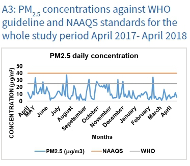
Table 1 presents the descriptive statistics of PM₂₅, soot, black carbon and UVPM determined throughout the sampling period (April 2017- April 2018). The PM₂₅ concentrations ranged from 1.06 to 37.52 μg/m³ with an average of 10.9 μg/m³. The PM₂₅ concentrations exceeded the daily WHO guideline of 25 μg/m³ on 9 occasions. However, the PM₂₅ concentrations were found to be within the South African National Ambient Air Quality Standard (NAAQS) of 40 μg/m³ (See appendix 3). Seasons were defined as followed: Autumn (18/4/2017 to 31/5/2017 and 1/3/2018 to 16/4/2018), winter (1/6/2017 to 31/8/2017), spring (1/9/2017 to 30/11/2017) and summer (1/12/2017 to 28/2/2018). The highest mean of PM₂₅ level was observed in spring and four exceedances of the daily WHO guideline were recorded, followed by autumn with two exceedances, while the highest mean levels of soot and BC was observed in winter followed by spring (Table 1). For UVPM, the highest mean level was observed in autumn followed by winter.

 

 

Higher concentration of PM_2.5 in spring is attributed to biomass burning prior to the onset of rainfall during September, which is followed by agricultural activities after the first rainfall in October and November resulting in daily WHO guideline exceedances. Biomass burning and agricultural activities have been identified as major contributors to PM₂₅ (DEA, 2009; Engelbrecht et al., 2002; DEA, 2012; Petkova et al., 2013; Hersey et al., 2015; Valsamakis, 2015; DEA, 2016; LEDET, 2016). High concentrations measured in winter are attributed to household warming during June and July and the prevalence of stable conditions in these months also contributes to the increase in concentrations. Stable conditions occur with little to no rainfall and calmer winds, as was observed in June and July (See Appendix 2). This results in longer atmospheric residence times of PM_2.5 and PM_2.5 chemical composition due to limited wet deposition and high accumulation of the aerosol properties (Perrino et al., 2011; Valsamakis, 2015). Low PM_2.5, soot, BC and UVPM levels in summer and autumn was due to unstable weather conditions. Unstable conditions are associated with high rainfall, increased wind speed. These conditions increase wet deposition and dispersion of PM_2.5, soot, BC and UVPM leading to low concentrations and less exceedances of the daily WHO guideline. Dependence on public transport during summer, and no household warming reduces PM₂₅, soot, BC and UVPM levels.

Correlation between PM₂₅ and meteorological variables

Table 2 presents the correlation coefficients and the corresponding p-values for the whole study period. Relative humidity and rainfall played a major role in decreasing PM_2.5 concentrations, due to the significant correlation. Relative humidity and rainfall decrease the concentration of PM_2.5, as deduced from negative correlation. PM_2.5 decreases with high relative humidity due to hygroscopic growth (Wang and Ogawa, 2015) rendering the particles to be too heavy to stay suspended in the atmosphere, also particulate matter act as condensation nuclei, during cloud formation as humidity increases. Significant negative relationship with rainfall, is due to wet deposition as atmospheric washout takes place when rainfall increases. High relative humidity and rainfall were measured in summer and autumn when compared to winter and spring and this negative relationship explains why winter and spring had high concentrations compared to summer and autumn. Wind speed was positively correlated with PM_2.5. Prevailing wind transports PM_2.5 from nearby sources to the receptor, and thus, as wind speed increases the PM₂₅ increases.

 

 

Temperature has shown an insignificant negative correlation. A study by Wang and Ogawa (2015) has also shown that high temperatures hindered formation of particles in summer. According to Tai et al., (2010) sulfate concentrations are expected to increase with increasing temperatures due to faster SO₂ oxidation, while semi-volatile components such as nitrates and organics are expected to decrease as they shift from particle phase to gas phase at high temperatures. Temperature has a decreasing and an increasing effect; in the case of Thohoyandou it had a decreasing effect due to high temperatures. This can be seen from high concentration in winter where low temperature was measured and low concentrations in summer where there was high temperature.

Chemical composition analysis

 

Elemental composition

Figure 3 and 4 presents the seasonal variations of elements detected in PM_2.5 in the air mass passing through Thohoyandou, in summer and autumn respectively. For each season two graphs were plotted one with high elemental concentrations and one with low elemental concentrations. The transition metals (Cr, Mn, Co, Ni, Cu, W, Zr, Au and Pd), alkali earth metals (Rb and Na), alkaline earth metals (Mg and Ca), other metals (Al, Bi, Ga and Sn), semi metals (Si, Ge, Sb and As), non-metals (S and Se) and halogens (I) were detected in the particulate matter (See appendix 4). In summer, 24 elements were detected and decreased monthly throughout the season. Higher concentrations of Na, Sb, Pd and Sn were measured followed by Mg, Si and S (Fig 3a). High concentrations of Na can be attributed to gusty winds and torrential rain brought by tropical cyclones from Indian ocean in summer. The elements with high concentrations are associated with long range transport (Pd, Sn, Sb) from the igneous bushveld complex, followed by the elements associated with crustal materials (Mg, Al, Si) and lastly elements from industrial activities (Cu, As, Co, Ni). The low concentrations of elements associated with crustal materials can be explained by the fact that the sampling period was also associated with rainfall, and thus the soil re-suspension was suppressed, and the dust was not easily suspended from the surface to become airborne while for industrial activities is due to limited industrial activities in Thohoyandou. The decrease in high concentration of the trace metals as the sampling period progresses is attributed to the fact that the beginning of the sampling was associated with unstable conditions, which facilitates dispersions and thus the high concentrations of these trace metals are highly dispersed. In autumn the high concentrations were Pd<Sn<S>Si. The concentrations of elements in autumn has decreased (Figure 4) this is attributed to increase in rainfall in this season which has scavenging properties. The concentrations of elements associated with crustal materials (Ca, Si, Mg) and Na significantly decreased in autumn this is because rainfall increased although the tropical cyclone season has passed, while Sn and Pd remained high as compared to other elements. Cr and Mn increased from February to April, the increase in these elements from industrial activities in autumn is attributed to change in backward trajectories which was dominated by Indian ocean origin in summer, wherein autumn has 25% backward trajectories originating from Zimbabwe picking up particles from industrial activities. A study by Hsu et al., (2016) has observed an abundance of Al followed by Ca, Mg, Fe and Zn in PM₂₅. This trend can be justified by the high rainfall during the sampling season, which suppress the soil and prevent dust re-suspension.

 

 

 

 

Morphological Analysis

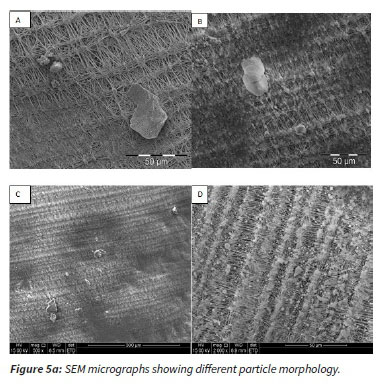
Figure 5(a) depicts the micrographs of particulate matter collected during 2017/2018 sampling period. In this study different kinds of morphologies were observed irregular, flat, and spherical (Figure 5a). Particles collected are clearly visible in the micrographs. A variety of particles shapes were observed from nearly perfect spherical shape to irregular shapes. The morphologies are consistent with the study by Li et al., (2019), wherein they observed irregular, flocculent, flat, rectangular, spheroidal, spherical, and regular particles. The shape of the particles is mainly depended on the source of the particles. Morphology and composition of these particles as done in previous studies (Van Zyl et al., 2014; Satsangi and Yadav, 2014) can help in identification of their sources. According to Van Zyl et al., (2014) the shapes of particles can be used to distinguish between windblown particles and anthropogenic particles. Well-rounded shapes are associated with anthropogenic sources, while unevenly shaped particles with natural sources. The particles in these micrographs are likely to be originating from natural emissions. As noted by Satsangi and Yadav (2014) PTFE filter is causing uncertainties because of its fiber structure observed from (Figure 5A).

 

 

In addition to visual inspection, EDS analysis was used to obtain the surface chemical composition. Figure 5b presents the micrograph of particulate matter and the subsequent chemical analysis of individual particles using EDS. The EDS as can be seen from the bar graphs (figure 5b) show the presence of Na, Mg, Al, Si, S, Cl, K, Ti, Cr, Fe. Majority of these oxygen-rich elements (Na, Mg, Al, Si, Cl, K, Ti, Cr, Fe) have been associated with natural sources such as crustal minerals erosion and surface winds, natural burning and from the oceans (Van Zyl et al., 2014). Additionally, a non-metallic species S, was detected, which suggests anthropogenic source. Flat particles and irregular (Figure 5b; Spectrum 1 and 4 respectively) comprises of C, O, Na, Mg, Al, Si, Ti, and Ca, these particles represent the crustal material. This type of particle primarily contained Si, Al, O, which is the elemental composition associated with phyllosilicates (AlSi)₃O₄. Spherical particles (Figure 5b: Spectrum 2) comprise of C, O, Na, Mg, Si and K. High content of C and K, show that its organic material and it was formed during biomass burning. Spheroid particles (Figure 5b: Spectrum 3), has shown additional elements such as Fe and S these morphologies represent industrial emissions.

Sources of elemental composition

Figure 6 presents the principal component and the subsequent elements. Principal component analyses identified seven principal components with even eigenvalues > 1 that explained 84.70% of the % variance in elemental composition sources (See appendix 5). The last one was not included in the discussion because it had one element even though it explained 4.93% of the total variance. The first component is comprised of Na, Mg, Si, Al, Sb, S, Ca, Zr, and soot. Mg, Al, Si, Ca has been linked with crustal materials throughout the literature (Zhang et al., 2008; Xia and Gao, 2011; Santanna et al., 2016; Yu et al., 2013; Zhang et al., 2013; Cheng et al., 2016) and thus component one is showing emissions from crustal material i.e. dust resuspension. crustal materials explained 24.21% of the total variance. The study conducted by (Mohammed et al., 2017; Sammaritano et al.,2018) this source had a high percentage of variance. Although this component has soot that has not been previously linked with crustal material in this study it was assigned mainly with crustal material because of the number of the elements associated with this component and the diversity of the source.

 

 

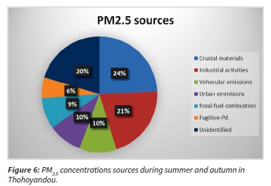
The second component is comprised of S, Ga, W, Bi, I, Ge, Au and Co. Zhang et al., (2008) linked S with coal combustion. Co has also been linked with combustion of fuel (Xia and Gao, 2011). W, Co, and Ga has been used in jewelries; Ga and Ge have been used in electrodes, while Bi and W has been used as alloys. This source has been attributed to industrial activities and has explained to 21.06% of the cumulative variance. The third component is comprised of Sb, soot, Co. Co has been linked with vehicular emissions (Rizzo and Scheff, 2007; Hsu et al., 2016) from batteries and gasolin. Sb was found to be from abrasion and brake wear (Xia and Gao, 2011) since it has been used in automotive brakepad. soot is known to originate from incomplete combustion of fossil fuel and thus, can be emitted from internal combustion engines more especially diesel engines through vehicles tailpipes. Vehicular emission explained 10.31% of total variance. The fourth component is comprised of Au, Cu, Rb, and Mn. Mn emissions are also linked to transportation activities such as tailpipe emissions, brake, and tire wear (Yu et al., 2013), refuse burning (Begum et al., 2007) resuspended soil dust (Cheng et al., 2015). Cu has been linked to industrial dust (Lee et al., 2008), vehicle exhaust (Yu, et al., 2013) and brake wear. This source has been linked to urban emissions and contibuted 9.56% of the total variance. The fifth component is comprised of Cr, BC, UVPM and Pd. BC has been linked with combustion processes (Engelbrecht et al., 2002). Combustion processes include fossil fuel combustion, diesel engine exhaust, as well as open biomass fires and household combustion (Chiloane et al., 2017). Cr has been linked to biomass burning (Yu et al., 2013; Zhang et al., 2013). Some coal fired power stations are also located in Limpopo where fossil fuels are burned continuously to generate electricity, the use of firewood and agricultural burning also take place. This source has been attributed to a mixture of fossil fuel combustion and has contributed 8.76% of the total variance. The sixth component is comprised of Sb and Pd. This source has been attributed to fugitive Pd and explained 5.80% of the variance. Pd is emitted from mining activities in the bushveld igneous complex (Schouwstra et al., 2000). The approximate sources of PM_2.5 in Thohoyandou during summer and fall are crustal materials re-suspension (24.21%), industrial emissions (21.06%) vehicular emission (10.31%), urban emission (9.56%); fossil fuel combustion (8.76%) and fugitive-Pd (5.80%).

Long range transport clusters

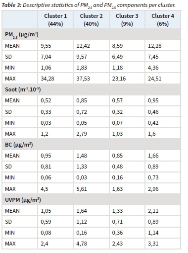
The clustered backward trajectories are presented in Figure 7 and the corresponding descriptive statistics per cluster are presented in Table 3. Four clusters were used in response to change in total spatial variance (TSV) as clusters are combined (Figure 7A). The clusters are from the Indian Ocean, Inland and recirculation. Cluster 2 (40%) and cluster 4 (6%) are associated with days of high PM_2.5 concentrations (Table 2). The high concentrations of these clusters can be explained by the fact that they are mainly inland, where there are many industrial activities. Cluster 2 is associated with air masses from Mozambique, although they occurred 40% of the time it was associated with days of high concentrations. Hersey, et al., (2015) observed that biomass burning emissions from Mozambique and Zimbabwe reach South Africa. A report by the Department of Environmental Affairs (DEA, 2009) indicated that biomass burning accounts for 20-40% of PM_2.5 concentration, and this explains the high concentration of PM_2.5 associated with air parcels that pass-through Mozambique. Cluster 4 is associated with air parcels from Botswana. DEA, (2009) points that among the air parcels that reach South Africa, there is an Indian plume, Atlantic plume and African plume. It was found that the African plume was associated with high pollutants. This explains the high concentrations associated with cluster 4, which is associated with days that exceeded the daily WHO guideline. Cluster 1 and cluster 3 are of oceanic origin and concentrations were lower on these days. This is because there are fewer emissions over the oceans. Air parcels from the Indian Ocean bring low concentrations of pollutants (DEA, 2009). Cluster 3 spent a lot of time over the ocean and thus, no exceedance, while cluster 1 spent less time and passed through Mozambique this explains the exceedances associated with this cluster. The Mozambican cluster is once again associated with high concentration of PM₂₅. This emphasizes the high contribution of Mozambique to PM_2.5 concentration in South Africa and shows that there are major sources of PM₂₅ in Mozambique that affect the South African air quality that need to be evaluated.

 

 

 

 

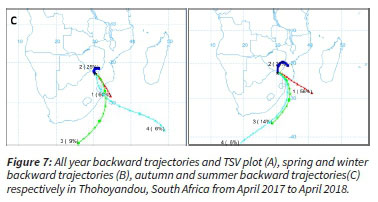
Spring season (Figure 7B left) has 82% (Cluster 1 44%, cluster 2 20% and cluster 3 18%) of backward trajectories originating Indian ocean passing through Mozambique 20% (cluster 2) of the 88% pass through Zimbabwe before reaching South Africa and 18% (cluster 4) of backward trajectories originating form Indian ocean reaching Thohoyandou. Besides different industrial activities these 3 countries have similar meteorological conditions with summer rainfall and spring onset rains and thus, biomass burning an agricultural activity in spring from all these countries has resulted in high concentrations in spring. Winter season (Figure 7B right) had 55% (cluster 1) of the backward trajectories closer to the receptor. This explains the high concentrations measured in winter due to limited dispersion, 8 % (cluster 2) of the backward trajectories were from Atlantic Ocean and passed through Lesotho and Mozambique before reaching South Africa. This is because south Africa also experiences Mediterranean climate, with cold fronts approaching from the west coast. And the reimaging 37% (cluster 3 and 4) originated from Indian ocean and passed through Mozambique before reaching the receptor.

Autumn season (Figure 7C left) had 69% (cluster 1 and 3) originating from Indian ocean passing through Mozambique, 6% (cluster 4) originating from Indian ocean and 25% originating from Zimbabwe reaching the receptor. Summer season (Figure 7C right) has 76% (cluster 1 ,3 and 4) of the clusters originating from Indian ocean passing through Mozambique, this explains the low concentrations measured in this season because tropical cyclones from Indian ocean not only control the prevailing winds but also brings the heavy rainfall with scavenging properties, and the remaining 24% cluster 2) originates in Mozambique pass through Zimbabwe before reaching South Africa. Precipitation has high decreasing effects, despite the similarities in the spring and summer cluster spring had the highest concentration measured while summer had the lowest concentrations.

 

Conclusion

This study presented the chemical characterization of PM_2.5 in Thohoyandou and further determined the sources of the PM_2.5 as well as the long-range clusters. The PM₂₅ concentrations were found to be ranging from 1.06 μg/m³ to 37.53 μg/m³ with the mean concentrations of 10.89 μg/m³ over the sampling period. The concentration of PM₂₅ was found to be higher than the daily WHO guideline on 9 occasions. The soot, UVPM and BC were found to be having an annual mean of 0.69 m^-1 10^-5, 1.40 μg/m³ and 1.22 |g/m³ respectively. The elemental analysis revealed the dominance of Pd, Sb, Sn, Mg, Al, Si elements. The source apportionment suggested that the PM₂₅ could be originating from Crustal materials, industrial, vehicular, urban and biomass burning emissions. HYSPLIT model showed that air parcel that pass-through Thohoyandou varies seasonally from four to six clusters. The results obtained showed that the air mass passing through Thohoyandou could pose some health effects on communalities living in the area. As such the study recommends the epidemiological studies assessing the health effects of PM₂₅ in Thohoyandou and more routine monitoring of PM₂₅.

 

Acknowledgements

The authors wish to acknowledge the South African Weather Service, for providing meteorological data.

This study was funded by the National Research Foundation grant (CPT160424162937; J. Wichmann was the PI; this study was part of a larger study that also included Cape Town and Pretoria) and supported by South African Department of Higher Education and Training Research incentive funds (W.M Gitari), University of Venda RPC (Grant G196), and NRF scholarship (R.J Novela).

The authors declare no conflict of interest.

 

Authors contributions

Novela Rirhandzu (student): Conceptualization, design of the study, data collection and writing - original draft. Gitari Mugera, Chikoore Hector: Supervision, resources, review and editing, funding acquisition. Molnar Peter: Resources, filter analysis for BC and UVPM. Mudzielwana Rabelani: Proof reading and revising manuscript. Wichmann Janine: Conceptualization, design of the study, supervision, resources, review and editing, funding acquisition.

 

References

Adeyemi, A., 2020. PM₂₅ chemical composition, source apportionment and geographical origin of air masses in Pretoria, South Africa. Pretoria: University of Pretoria.         [ Links ]

Begum, B., Biswas, S. & Hopke, P., 2007. Source Apportionment of Air Particulate Matter by Chemical Mass Balance (CMB) and Comparison with Positive Matrix Factorization (PMF) Model. Aerosol and Air Quality Research, 7(4), pp. 446-468. https://doi.org/10.4209/aaqr.2006.10.0021.         [ Links ]

CCAC, 2019. Black Carbon, https://www.ccacoalition.org/en/slcps/black-carbon:Climate_and_clean_air_coalation.         [ Links ]

Cheng, Y. et al., 2015. PM₂₅ and PM₁₀₂₅ chemical composition and source apportionment near a Hong Kong roadway. Particuology, 18, pp. 96-104. https://doi.org/10.1016/jj.partic.2013.10.003.         [ Links ]

Cheng, Y. & Yang, L., 2016. Characteristics of Ambient Black Carbon Mass and Size-Resolved Particle Number Concentrations during Corn Straw Open-Field Burning Episode Observations at a Rural Site in Southern Taiwan. International Journal of Environmental Research and Public Health. https://doi.org/10.3390/ijerph13070688.         [ Links ]

Chiloane, K. et al., 2017. Spatial, temporal and source contribution assessments of black carbon over the northern interior of South Africa. Atmospheric Chemistry and Physics, 17, p. 6177-6196. https://doi.org/10.5194/acp-17-6177-2017.         [ Links ]

DEA, 2009. State of Air Report 2005. A report on the state of air in South Africa, Pretoria: Department of Environmental Affairs.         [ Links ]

DEA, 2012. South Africa environment outlook: Air quality draft, Pretoria: Department of Environmental Affairs.         [ Links ]

DEA, 2016. 2nd South Africa Environment Outlook. A report on the state of the environment, Pretoria: Department of Environmental Affairs.         [ Links ]

Draxler, R. & Rolph, G., 2003. HYSPLIT (HYbrid Single-Particle Lagrangian Integrated Trajectory) model, Silver Spring: NOAA ARL READY website (http://www.arl.noaa.gov/ready/hysplit4.html).         [ Links ]

Engelbrecht, J.P., Swanepoel, L., Chow, J.C., Watson, J.G. and Egami, R.T., 2002. The comparison of source contributions from residential coal and low-smoke fuels, using CMB modeling, in South Africa. Environmental Science & Policy, 5(2), pp. 157-167. https://doi.org/10.1016/S1462-9011(02)00029-1.         [ Links ]

Freiman, M. & Piketh, S., 2002. Air Transport into and out of the Industrial Highveld Region of South Africa. Journal of Applied Meteorology, 42, pp. 994-1003. https://doi.org/10.1175/1520-0450(2003)042<0994:ATIAOO>2.0.CO;2.         [ Links ]

Hersey, S., Garland, R.M., Crosbie, E., Shingler, T., Sorooshian, A., Piketh, S. and Burger, R., 2015. An overview of regional and local characteristics of aerosols in South Africa using satellite, ground, and modeling data. Atmospheric Chemistry and Physics, 15, p. 4259. https://doi.org/10.5194/acp-15-4259-2015.         [ Links ]

Hsu, C., Chiang, H., Lin, S., Chen, M., Lin, T., Chen, Y., 2016. Elemental characterization and source apportionment of PM₁₀ and PM₂₅ in the western coastal area of central Taiwan. Science of the Total Environment, p. 1139-1150. https://doi.org/10.1016/j.scitotenv.2015.09.122.         [ Links ]

LEDET, 2016. Limpopo environmental outlook report, Polokwane: Department of Economic Development, Environment and Tourism Limpopo.         [ Links ]

Lee, S. Liu, W., Wang, Y., Russell, A.G. and Adgerton, E.S., 2008. Source apportionment of PM₂₅: Comparing PMF and CMB results for four ambient monitoring sites in the southeastern United States. Atmospheric Environment, 42, p. 4126-4137. https://doi.org/10.1016/j.atmosenv.2008.01.025.         [ Links ]

Li, Y. et al., 2019. Morphological characterization and chemical composition of PM_2.5 and PM₁₀ collected from four typical Chinese restaurants. Aerosol Science and Technology, pp. 11861196. https://doi.org/10.1080/02786826.2019.1645292.         [ Links ]

Mohammed, G., K. G. & Mitchell, D., 2017. Trace Elemental Composition in PM₁₀ and PM₂₅ Collected in Cardiff, Wales. Energy Procedia, p. 540-547. https://doi.org/10.1016/j.egypro.2017.03.216.         [ Links ]

Monlar, P., Tang, L., Sjoberg, K. & Whichmann, J., 2017. Longrange transport clusters and positive matrix factorization source apportionment for investigating transboundary PM_2.5 in Gothenburg, Sweden. Environmental Science Process and Impacts, 19, pp. 1270-1277. https://doi.org/10.1039/C7EM00122C        [ Links ]

Mzezewa, J., Misi, T. & van Rensburg, L., 2010. Characterisation of rainfall at a semi-arid ecotope in the Limpopo Province (South Africa) and its implications for sustainable crop production. African Journal Online, 36(1). https://doi.org/10.4314/wsa.v36i1.50903.         [ Links ]

Olaniyan, T., Dalvie, M. & Jeebhay, M., 2015. Ambient air pollution and childhood asthma: a review of South African epidemiological studies: allergies in the workplace. Current Allergy & Clinical Immunology, 28(2), pp. 122-127.         [ Links ]

Osidele, O., 2016. An Analysis of Patterns and Trends of Road Traffic Injuries and Fatalities in Vhembe District, Limpopo Province, South Africa. Thohoyandou: University of venda.         [ Links ]

Perrino, C. et al., 2011. Chemical characterixation of atmospheric PM in Delhi, India, during different periods of the year including Diwali festival. Atmospheric Pollution Research, 2, pp. 418-427. https://doi.org/10.5094/APR.2011.048.         [ Links ]

Petkova, E., Jack, D., Volavka-Close, N. & Kinney, P., 2013. Particulate matter pollution in African cities. Air Quality, Atmosphere & Health, 6(3), pp. 603-614. https://doi.org/10.1007/s11869-013-0199-6.         [ Links ]

Rizzo, M. & Scheff, P., 2007. Fine particulate source apportionment using data from the USEPA speciation trends network in Chicago, Illinois: Comparison of two source apportionment models. Atmospheric Environment, 41, p. 6276-6288. https://doi.org/10.1016/j.atmosenv.2007.03.055.         [ Links ]

Sammaritano, M., Bustos, D., Poblete, A. & Wannaz, E., 2018. Elemental composition of PM₂₅ in the urban environment of San Juan, Argentina. Environmental Science and Pollution Research, p. 4197-4203. https://doi.org/10.1007/s11356-017-0793-5.         [ Links ]

Santanna, F. et al., 2016. Elemental composition of PM₁₀ and PM_2.5 for a Savanna (Cerrado) region of Southern Amazonia. Química Nova, pp. 1170-1176. https://doi.org/10.21577/0100-4042.20160154.         [ Links ]

Satsangi, P. & Yadav, S., 2014. Characterization of PM 2.5 by X-ray diffraction and scanning electron microscopy-energy dispersive spectrometer: its relation with different pollution sources. International Journal of Environmental Science and Technology, 11(1), pp. 217-232. https://doi.org/10.1007/s13762-012-0173-0.         [ Links ]

Schouwstra, R., Kinloch, E. & Lee, A., 2000. A short geological review of the Bushveld complex. Platinum metals Review, 44(1), p. 33.         [ Links ]

SSA, 2012. Census 2011, Pretoria: Stats SA Library Cataloguing-in-Publication (CIP) Data.         [ Links ]

Tai, A., Mickley, L. & Jacob, D., 2010. Correlations between fine particulate matter (PM_2.5) and meteorological variables in the United States: Implications for the sensitivity of PM₂₅ to climate change. Atmospheric Environment, 44, pp. 3976-3984. https://doi.org/10.1016/j.atmosenv.2010.06.060.         [ Links ]

Tang, L. et al., 2014. Estimation of the long-range transport contribution from secondary inorganic components to urban background PM₁₀ concentrations in south-western Sweden during 1986-2010. Atmospheric Environment, 89, pp. 93-101. https://doi.org/10.1016/j.atmosenv.2014.02.018.         [ Links ]

Valsamakis, S., 2015. Ambient air quality monitoring: a comparison between two urban parks in Soweto, South Africa. Johannesburg: University of Witwatersrand.         [ Links ]

Van Zyl, P. et al., 2014. Assessment of atmospheric trace metals in the western Bushveld Igneous Complex, South Africa. South African Journal of Science, 110(3/4). https://doi.org/10.1590/sajs.2014/20130280.         [ Links ]

Wang, J. & Ogawa, S., 2015. Effects of Meteorological Conditions on PM₂₅ Concentrations in Nagasaki, Japan. International Journal of Environmental Research and Public Health, 12, pp. 9089-9101. https://doi.org/10.3390/ijerph120809089.         [ Links ]

WHO, 2014. Seven million premature deaths annually linked to air pollution, http://www.who.int/mediacentre/news/releases/2014/air-pollution/en/:WHO.         [ Links ]

WHO, 2016. Sustainable Development Goals: Health and Health Related Targets, http://www.who.int/gho/publications/world_health_statistics/2016/EN_WHS2016_Chapter6.pdf:WHO.         [ Links ]

Wichmann, J. et al., 2014. The effect of secondary inorganic aerosols, soot and the geographical origin of air mass on acute myocardial infarction hospitalisations in Gothenburg, Sweden during 1985-2010: a case-crossover study. Environmental Health, 13(1), p. 61. https://doi.org/10.1186/1476-069X-13-61.         [ Links ]

Xia, L. & Gao, Y., 2011. Characterization of trace elements in PM₂₅ aerosols in the vicinity of highways in northeast New Jersey in the U.S. east coast. Atmospheric Pollution Research, pp. 34-44. https://doi.org/10.5094/APR.2011.005.         [ Links ]

Yu, L. et al., 2013. Characterization and Source Apportionment of PM_2.5 in an Urban Environment in Beijing. Aerosol and Air Quality Research, 13, p. 574-583. https://doi.org/10.4209/aaqr.2012.07.0192.         [ Links ]

Zhang, R., Fu, C., Han, Z. & Zhu, C., 2008. Characteristics of elemental composition of PM₂₅ in the spring period at Tongyu in the semi-arid region of Northeast China. Advances in Atmospheric Sciences, p. 922-931. https://doi.org/10.1007/s00376-008-0922-7.         [ Links ]

Zhang, R. et al., 2013. Chemical characterization and source apportionment of PM_2.5 in Beijing: seasonal perspective. Atmosperic Chemistry and Physics, Volume 13, p. 7053-7074. https://doi.org/10.5194/acp-13-7053-2013.         [ Links ]

 

 

Received: 5 August 2020
Reviewed: 14 September 2020
Accepted: 5 October 2020

 

 

* gitariw@gmail.com

 

 

Appendix

A1: Gravimetric analysis

A1.1 Weighing procedure: reference and sample filters

1. Download logged data from data-logging environmental monitor

2. Check if environmental conditions in the laboratory was maintained for the previous 24 hours within the prescribed limits

- Dry air temperature = 21 ± 1.0°c

- Relative humidity = 50 ±5%

3. Record environmental conditions immediately prior to weighing reference filters

4. Ensure balance is level

5. Weigh a mass of 2 grams repeatedly until repeatability is reached

6. Close balance doors and tare the balance

7. Open the balance doors and place three refence (control) filters on the weighing grid. Note: use 3 reference (control) filters for each 10 sample filters.

8. Close balance doors and start count down timer

9. Allow 30 seconds for balance to stabilize

10. Note reading on the balance immediately when settling time has expired

11. Remove reference (control) filters from the weighing chamber and hold it next to the weighing chamber. Take care not to breath over the filters

12. Close the balance door and wait for balance to return to zero

13. If balance does not return to zero:

- Discard all weighing results

- Inspect the balance pan for dust or any other obstacle

- Tare the balance

- Reweigh filters

- Balance should not otherwise be tarred between weighing filters

14. Follow steps 7-13 to obtain 3 consecutive weights for the 3 reference (control) filters

15. Proceed to weigh 10 individual sample filters by following the above procedure (steps 7-13)

16. After weighing the 10 sample filters, weigh the 3 reference filters again using steps 7-13

17. Record environmental conditions immediately after weighing reference filters

18. If the maximum and minimum weight of reference filters differ more than 1% from average, discard results and re-weigh

19. Place weighed filters with a clearly marked support pad in a clean filter cassette holder

A1.2 Measuring concentrations

After sampling filters were conditioned for 24 hours and weighed under the same conditions.

Mass of the particulate matter was calculated using the same formulae:

M_pm= mass of the particulate matter, m_o= initial mass of the filter, m_f= final mass of the filter, m_b= mass of the blank filter.

The volume of air sampled was calculated using the following formulae:

V_a= volume of the air sampled, Q_ave= average flow rate, t = time elapsed.

Then the concentration of PM_2.5 was calculated using the following formula:

EEL43 reflectometer was used to measure soot. Absorption coefficients (prosy for soot) was expressed in m^_110^-5 (SOP RUPIOH 4.0, 2002) calculated using the following formulae:

(A-The loaded filter area, V-sampled volume, Ro-reflection of primary control filter, Rs-Reflectance of the sampled filter).

ATNIR and ATN UV were measured using a Model OT21 Optical Transmissometer (Magee Scientific Corp., Berkeley, California, USA). Thereafter used to calculate BC and UVPM using the following formulae;

The elemental mass concentration obtained from wavelength dispersive X-ray fluorescence (WD-XRF) spectrometer (PANALYTICAL AXIOSMAX) analysis given in μg.cm^-2 and converted to μg.m^-3 using the following formulae:

EM = elemental mass concentration, EM_f= elemental concentration of the exposed filter, EM_belemental concentration of blank filter.