RESEARCH ARTICLE

 

Source profiling, source apportionment and cluster transport analysis to identify the sources of PM and the origin of air masses to an industrialised rural area in Limpopo

 

 

Cheledi Tshehla^{I, II}; George Djolov^{I, †}

^IDepartment of Geography, Geoinformatics and Meteorology, University of Pretoria, Pretoria, South Africa
^IISouth African Weather Service, Centurion, Gauteng, South Africa, cheledi.tshehla@weathersa.co.za

 

 

---

ABSTRACT

The Greater Tubatse Municipality in Limpopo is home to three ferrochrome smelters and over fifteen operational mines which are mining chromium, platinum or silica. Source apportionment in this study was performed by combining air mass back trajectories and receptor modelling. The particulate matter (PM) samples at six sites were collected using the University of North Carolina Passive Samplers. The monthly samples were collected for a period of 4-5 weeks, except for August-September and September-October 2015 where the samples were collected for up to 6 weeks. The sampling was carried out from July 2015 to June 2016. PM chemical analysis was performed using Computer Controlled Scanning Electron Microscopy coupled with Energy-Dispersive X-ray Spectroscopy (CCSEM-EDS). The PM chemical analysis indicated the presence of elements such as carbon (C), calcium (Ca), chromium (Cr), iron (Fe), aluminium (Al), silicon (Si), magnesium (Mg) and lead (Pb). All the six sites except site 1 exceeded the WHO annual guidelines for PM₁₀ concentration of 20 µg/m^-3. The annual chromium concentrations exceeded the New Zealand limits of 0.0001 µg/m^-3 and 0.11µg/m³ Cr (VI) and Cr (III), respectively. The back trajectory clusters computed by the HYSPLIT model identified 5 transport clusters for each site. The main transport patterns were northerly to north-easterly, easterly to south-easterly, and south-westerly to north-westerly. The US EPA PMF model version 5.0 used in source profiling and source apportionment identified agriculture/wood combustion, coal combustion, crustal/road dust, ferrochrome smelters, and vehicle emissions as the main sources in the area. The source contributions varied across all sites indicating the existence of different microenvironments within the airshed and that the pollution can originate from either local or regional sources as indicated by back trajectory clusters.

Keywords: source apportionment, back trajectories, particulate matter, chemical characterization.

---

 

 

Introduction

South Africa is one of the developing countries in the world, and as such the country has considered economic growth, social and educational development and industrialization as key development priorities. In the Greater-Tubatse Municipality (GTM) in Limpopo Province, South Africa, mining is viewed as one of the important economic activities which has the potential of contributing to the development of the area's economy (Community Empowerment Impact Assessment Report, 2007). Though the contribution of mining activities to economic development of GTM is well acknowledged, this might be achieved at a significant environmental, health and social costs to the region due to urbanization, high traffic volumes and higher industrial and domestic waste production.

Environmental pollution due to heavy metals from mining activities, vehicular emissions, agricultural and biomass burning are a major concern in many parts of the world (UNEP, 2006). Extensive mining of chromite, platinum and silica in the GTM mining belt may pose a serious threat to the environment. Mining of these ores may release toxic metals such as hexavalent chromium and platinum group metals which are carcinogenic and mutagenic to human health (Zayed and Terry, 2003; Ravindra et al., 2001). Studies worldwide have found that ambient levels of PM₁₀ are associated with adverse health effects including increase in premature deaths, hospital admissions and emergency attendances for respiratory and cardiovascular disease and exacerbation of asthma (Pope III, 2000; Dockery, 2001). PM_2.5 which is smaller in aerodynamic diameter than PM₁₀, can penetrate deeper into the lungs and reach the blood system and it can also impact on visibility and climate change (Chen et al., 2014) The potential of adverse health effects of particulate pollution has triggered extensive research on PM chemical composition and source apportionment in many countries over the past decade (Liu et al., 2018). Understanding the chemical components of PM is crucial to adequately assess the impacts of these chemicals on the receiving environment. A number of ferrochrome smelters are found in the GTM. Ferrochrome is a major chromium source used as raw material for the production of stainless steel and ferro-metal alloys. The morphology of the chromite spinel ore can be described stoichiometrically as (Fe²⁺, Mg²⁺)O.(Al³⁺, Cr³⁺, Fe³⁺)_2∙O₄ and they often contain gangue compounds of SiO₂ and MgO. Submerged-arc furnaces are commonly used to smelt chromite ores by using carbonaceous reductants such as coke, bituminous coal and char. The ferrochrome slag created during the smelting process mainly consists of SiO₂, Al2O₃ and MgO in different proportions but also smaller amounts of CaO, chromium and iron oxides (Nkohla, 2006; Hockaday and Bisaka, 2010). These elements may find their way into the atmosphere during the smelting operations and they can cause serious harm to human health.

In South Africa, the National Environmental Management: Air Quality Act (AQA, Act No. 39 of 2004) was promulgated in 2005 as an approach to manage air quality in the country. The Act requires national, provincial and local authorities to identify substances or mixtures of substances in ambient air which may reasonably be anticipated to endanger public health, and to establish air quality standards to limit emission of such substances. However, to date no ambient metal standards (with the exception of Pb) have been promulgated to define the level of air quality that is necessary to protect the public welfare from known or anticipated adverse effects of these pollutants on the receiving environment in South Africa. There is also little information on PM source apportionment studies to assist in developing effective policies to mitigate the impacts of PM in South Africa.

Numerous methods have been developed over the years to collect and analyze air pollutant samples, using both active and passive techniques. Easy to use passive samplers are available in the market and are less expensive than conventional samplers. Therefore, a large number of passive samplers can be deployed at a given time to capture representative spatial measurements in an airshed (Lagudu et al., 2011).

There are two types of models (source-oriented models and receptor models) used to identify sources of pollution in the environment (Schauer et al., 1996). Source-oriented (dispersion) models require knowledge of all emissions from the contributing sources (Pant and Harrison, 2012). Receptor modes are statistical analysis tools used to identify contributions from different sources using multivariate measurements from different receptor locations. These models use ambient data and the chemical components in source emissions to quantify contributions, unlike the source models that use emissions and meteorological parameters to estimate concentrations at the receiving environment (Watson, 2002). Positive Matrix Factorization (PMF) is one of the recent models developed by the United State (U.S) Environmental Protection Agency (EPA). PMF has been used widely in source apportionment of ambient PM because of its ability to account for the uncertainty variables that are often associated with sample measurements and also the output values in the solution profiles and contributions are nonnegative (Reff and Eberly, 2007). The key output of PMF is the percentage contributions of different sources to ambient pollutant concentration at specific receptors (Pant and Harrison, 2012). The PMF model has been used by many researchers across the world for source identification and profiling. A study by Harris and Davidson (2005) characterized Ca, Al, Mg, Si, K, Fe, Mn and Zn as elements emitted from metal smelters. Soil was found to contain elements such as Fe, Al, K, Ca, Ti in a study by Watson and Chow (2001a; 2001b), while road dust contributed to Fe, Al, K, Ca, Si, Mg, P, S, Na and BC (Bhave et al., 2001; Ho et al., 2003). However, these profiles can vary from one area to the other due to varying soil types. A source profiling study by Kim et al., (2003b) and Begum et al., (2004) identified motor vehicle emissions as the source of Mg, Al, Fe, Si, S and BC (black carbon). Biomass burning emissions are a mixture of both organic carbon and elemental carbon and their ratio depends on the type of fuel used (Karanasiou et al., 2015).

The quantitative assessment of sources contributing to the ambient PM on the receiving environment is required to develop sound and effective control strategies to address the scourge of PM pollution in South Africa. However, the bottom-up approach based on emission inventories is hindered by poor availability of the emissions data particularly from industries. The objective of this study is to identify sources of PM in a mountainous terrain in Limpopo, South Africa and estimate their contributions through receptor modeling (PMF) application. The sampling data obtained during the sampling campaign from July 2015 to June 2016 will be used.

 

Methods

Study area

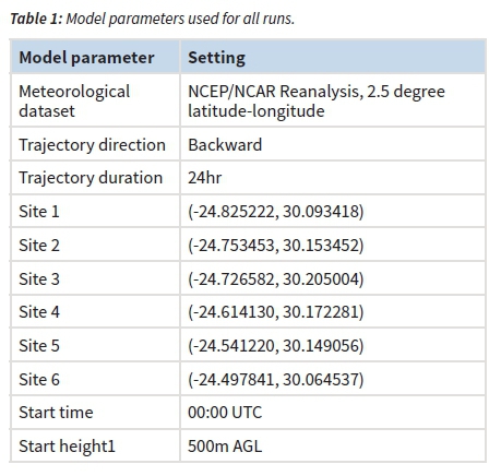
Ambient PM sampling was undertaken in a rural area of the Greater Tubatse Municipality (GTM) in Limpopo Province, South Africa (Fig. A1). The main towns in the area are Steelpoort and Burgersfort which are sustained through economic activities such as mining and smelting of chromium ores. Furthermore there are agricultural and forestry activities and transportation that also add to the economic activities in the area. Most of the households in the area are dependent on wood burning for space heating and cooking (Community Empowerment Impact Assessment Report, 2007). The GTM has a complex terrain with high mountains and steep inclinations. The elevation of the surface area is approximately 740 m above sea level with the surrounding mountains extending to a height of approximately 1200-1900 m above sea level. The area is located in the subtropical climate zone where the maximum average temperature reaches 35 °C with minimum average temperature of 18 °C in summer. In winter the maximum average temperature reaches 22 °C with average minimum of 4 °C (Schulze, 1986). The annual rainfall for the area ranges between 500 and 600mm (DWAF, 2005). Figure A1 in appendix shows the map of the study area showing passive sampler locations (red place-marks on Google map), with smelters shown as green place-marks.

Site selection

The location of the monitoring sites was selected to optimize spatial sampling for exposure assessment. A sequential sampling technique (Goovaerts, 1997; Van Groenigen et al., 1997) was used to design an optimal sampling network of 6 sites in the GTM. This technique is based on extended knowledge of the area to be sampled and factors controlling the distribution of pollutants. These factors amongst others were terrain and various phenomena like meteorological conditions and the chemistry of pollutants (Frączek et al, 2009). The sites were located at private residences, a church, a hospital and a school for security reasons and easy access during site visits.

Sampling and sample analysis

The University of North Carolina (UNC) passive samplers designed by Wagner and Leith (2001) and housed in a protective shelter designed by Ott and Peters (2008) were deployed at six sites for PM sampling. Ott and Peters (2008) designed the shelter to shield the passive sampler from precipitation and to minimize the influence of wind speed on particle deposition (Sawvel, 2015). The samplers consist of a scanning electron microscopy (SEM) stub, a collection substrate, and a protective mesh cap (Lagudu et al., 2011). The samplers were deployed for sequential periods of approximately 30 days from July 2015 to June 2016, except for the month of August and September when they were deployed for a period of approximately 40 days. The longer sampling periods of 3-4 weeks were selected to ensure that there was sufficient particle loading on the samplers as suggested by Sawvel (2015).

The PM_2.5, PM₁₀ concentrations and the elemental composition of individual particles deposited on the passive sampler were determined by CCSEM-EDS (Tescan Vega 3 model). Before sample analysis with Personal Scanning Electron Microscopy (PSEM) (method by Hopke and Casuccio, 1991), the samples were coated with a thin layer of graphitic carbon under vacuum to bleed off the charges induced by the electron beam in the SEM. The PSEM was operated with a 20-kV beam (Sawvel 2015). Lagudu et al., (2011) gave a brief description of the CCSEM analysis. The elements obtained from the analysis were Carbon (C), Chromium (Cr), Calcium (Ca), Iron (Fe), Silicon (Si), Aluminium (Al), Magnesium (Mg), Lead (Pb), and other miscellaneous elements. Pb and miscellaneous elements were not included in further analysis due to their insignificant weight. The concentrations of PM_2.5, PM₁₀ and each particle was determined using the method outlined in Ott and Peters (2008). Data obtained from CCSEM is semi-quantitative, and therefore, in order to use the data in PMF for source contributions the particles needs to be classified into homogenous groups by applying cluster analysis (Song and Hopke, 1996b; Kim and Hopke, 2008; Lagudu et al., 2011).

Cluster analysis

Buhot et al., (1999) described cluster analysis in detail. In this study, hierarchical cluster analysis was performed on single particle data from CCSEM using the open source clustering software (Cluster 3) developed by the Institute of Medical Science (IDS) at the University of Tokyo. Once the analyses were completed, all the cluster groups with less than 4 (excluding Pb and miscellaneous elements) particles were chosen as potential homogenous classes. This is because as the number of classes created for each source sample increases, the number of particles assigned to each class decreases (Kim and Hopke, 1988). The particle classes obtained from cluster analysis include Carbon-rich (C-rich), Chromium-rich (Cr-rich), Iron-rich (Fe-rich), Iron/Chromium-rich (FeCr-rich), Silicon (Si-rich), Silicon/Aluminium/Iron-rich (SiAlFe-rich), Calcium-rich (Ca-rich), Silicon/Magnesium-rich (SiMg-rich) and Silicon/Aluminium-rich (SiAl-rich).

Positive matrix factorization

PMF 5.0 (USEPA, 2014) was used to apportion the contribution from emission sources (Lee et al., 1999; Reff et al., 2007). The guidelines specified in the user manual were closely followed in this study. Two input files are required by the model: the sample species concentration values and the sample species uncertainty values or parameters for calculating uncertainty. In this study, the sample species uncertainties were obtained during CCSEM analysis of samples.

The receptor modelling in principle relies on the observed concentrations of chemical species in the atmosphere and these species must be conserved during transport between the source and the receptor. The conserved mass is then used during the analysis in the identification and apportionment of these species (Pant and Harrison, 2012). The PMF model identifies the sources by applying the following mass balance equation:

Where x_ij is the concentration of the j^th species in the i^th sample, g_ik the contribution of k^th source to the i^th sample, f_kj the concentration of the j^th species in the k^th source, and e_ij is the difference between the measured and fitted value. If the number and sources in the area being modelled are known, (f_kj), then the mass contribution of each source to each sample, g_ik, in equation (1) is known (European Commission, 2014). However, the objective is to calculate values of g_ik, f_kj, and p that can reproduce x_ij. An adjustment is then made to g_ik and f_kj until the minimum value of Q for a given p is found. Q is defined as:

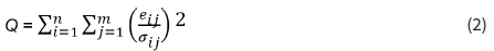
Where σ_ij is the uncertainty of the j^th species concentration in sample I, n is the number of samples, and m is the number of species (Reff et al., 2007). In most cases, a given chemical constituent will have multiple sources and the program performs correlation analysis to generate chemical profiles of 'factors' characteristic of the sources. Past knowledge of source chemical profiles is then used to assign factors to sources (Pant and Harrison, 2012). However, in South Africa there are few source chemical profiles available. Therefore, the international source chemical profiles (Central Pollution Control Board Parivesh Bhawan, East Arjun Nagar Delhi; Pant and Harrison, 2012; Barrera et al., 2012) were used as a guide.

HYSPLIT model

Backward air trajectories arriving at the six sampling sites were calculated using the Windows PC version of the Hybrid Single Particle Integrated Trajectory (HYSPLIT-4) model. This model is a system for computing air mass trajectories and complex dispersion and deposition simulations (Draxler and Hess, 1997; 1998). Meteorological data fields to run the model are available from routine archives. In this study, 24-hour back trajectories were calculated at a height 500 meters above ground level using reanalysis data from National Centre for Environmental Prediction (NCEP) and National Centre for Atmospheric Research (NCAR) available from the National Oceanic and Atmospheric Administration's (NOAA) Air Resources Laboratory (ARL) archives. The reanalysis data covers the globe from 1948 to the present with a horizontal resolution of about 2.5 x 2.5 degrees latitude-longitude and with an output every 6- hours.

The isosigma vertical motion method was selected for computing trajectories. This method follows the internal terrain following coordinates systems. A review on computation and applications of trajectories was provided by Stohl (1998). The length of the back trajectories is restricted in many ways by the distances between source regions and the destination zone. The choice of 24-hour back trajectory duration is a compromise between the objective to identify local and distant sources and sink regions and to limit the uncertainties in the trajectories. Stohl (1998) affirmed that errors of 20% of the distance travelled seem to be typical for trajectories computed from analysed wind fields.

Trajectory cluster analysis

In this study trajectory cluster analysis was performed using the HYSPLIT_4 model. The model uses Ward's method described by Romesburg (1984), Moody and Galloway (1988) and Stunder (1996). The HYSPLIT clustering method is described in detail by Draxler et al., (2018). Five clusters were chosen for each set of trajectory end point files because this number was sufficient to identify all major flow patterns, as well as several less common but nonetheless important patterns. Once the number of clusters has been decided, 'Special Runs' was chosen as the technique to produce standard clusters for all trajectory end points for the period starting from July 2015 to June 2016. A practical advantage of 'Special Runs' it's its ability to accommodate large volumes of data. The variables clustered were the latitude and longitude of trajectory segment endpoints at 1-hour intervals along each 24-hour back trajectory. Individual trajectories were further averaged to produce "cluster-mean" trajectories. Thus, our large data base (annual trajectories) was reduced to a number of cluster-mean plots that can be interpreted in terms of known mesoscale and synoptic features. For each cluster, ensemble plots of all individual trajectories belonging to that cluster were produced. These ensembles or "cluster membership" plots were used to validate the mean and to assess the variability within the cluster (HYSPLIT4, 2018).

 

 

Results and discussion

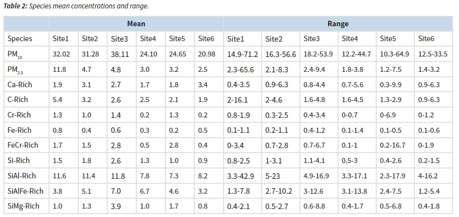
The mean annual concentrations and the range between minimum and maximum concentrations for PM_2.5, PM₁₀, and particle classes obtained through cluster analysis are shown in Table 2. The PM_2.5 and PM₁₀ annual mean concentrations were below the South Africa National Ambient Air Quality Standard (NAAQS) of 20 µg/m³ and 40 µg/m³_, respectively. However, all the sites exceeded the WHO annual guideline of 20 µg/m³ for PM₁₀ and only site 1 exceeded the WHO annual guideline of 10 µg/m³ for PM_2.5 (WHO, 2017). All the sites with the exception of site 4 and 6 recorded highest maximum PM₁₀ concentration above 50 µg/m³ with the minimum concentration of 10.3 µg/m³ recorded at site 5. For chromium, all sites exceeded the New Zealand annual chromium limits (Ministry for the Environment, 2009) of 0.0011 µg/m³ and 0.11 µg/m³ for Cr (VI) and Cr (III), respectively. This is an indication that the area may experience negative impact on human health, and because the pollutants' toxicity differs so should be the environmental regulation strategies to mitigate their impacts. The existence of SiAl-rich particles with concentrations ranging between 3.3 µg/m³ and 42.9 µg/m³ in the study area may result in cardio metabolic effects on animals and humans (Sun et al., 2012) because they contribute 15%-55% of the total PM in the study area.

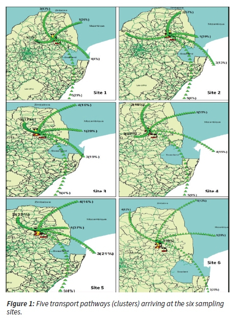
HYSPLIT transport clusters

Figure 1 shows five clusters per receptor site. Clusters for site 1 to site 4 have similar pattern with varying trajectory percentage. For site 1, cluster 1 with 36% of trajectories originates from Mozambique and arrives at the receptor site by passing through mining areas and a smelter northeast of the sampling site. Cluster 2 with 12% of the trajectories originates from Zimbabwe and arrives at the receptor site from the northwest and away from the mines and smelters in the area. Cluster 3 with 20% of trajectories originates from the west while clusters 4 and 5 originate from the Indian Ocean. Only cluster 1, 4 and 5 pass through areas with mines and smelters within the study area. This makes them potential transporters of heavy metals to the receptor site. For site 2, all clusters with the exception of cluster 4 passes over the mines and smelters and as such have the potential of carrying elemental particles to the site. For site 3, all the clusters pass over the mining areas and only cluster 3 and 5 passes over the smelters. Hence all these clusters can transport elemental particles to the receptor. For site 4, all the clusters pass over mining areas and only cluster 2 and 3 pass over the smelters before arriving at the receptor site. For site 5, only cluster 1 is not passing over any industrial facility in the area. For site 6, only cluster 2, 3 and 5 pass over industrial facilities. Cluster 2 with 30% of trajectories is recirculating within the vicinity of the receptor site and this makes it the most likely contributor of local pollutants. However, it should be noted that even though some trajectories are not passing through the industrial facilities, they can also transport pollutants from a variety of sources such as transport, agriculture, domestic, crustal and oceans, and that these pollutants also contribute to the observed concentrations as shown in Table 2.

 

 

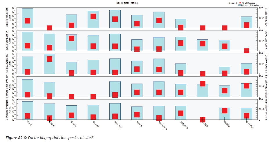
Source profiling by PMF

The most important step in PMF is to determine the number of factors which correspond to potential particle sources. After applying bootstrap and displacement tests on the data sets, three to five factors were deemed to be appropriate for a five source solution. The profile graph (Fig. A2.1-A2.6) displays the mass of each species apportioned to the factor (blue bar) and the percentage of each species apportioned to the factor (red bar). The factors were identified according to the type of elements dominating in percentage in that factor. Agricultural/wood combustion was associated with the dominance of C as a primary species and Fe elements. Ferrochrome smelter was identified by the domination of Cr and Fe elements. Crustal/road dust factor was associated with Si, Al, Ca and Mg as the primary elemental species. Industrial coal combustion factor was identified by Ca, C, Al and Si as the dominating elements. Vehicular emission factor was associated with Fe as the primary species, C, Al, Si, and Ca. The most interesting outcome is that Cr was also associated with crustal/road dust and agricultural/wood burning which is an indication that once this element is emitted from the source it is then deposited on to the soil and water bodies before it is absorbed by plant material and released into the atmosphere during burning. Figures A2.1-A2.6 in the appendix show the factor fingerprints for the species.

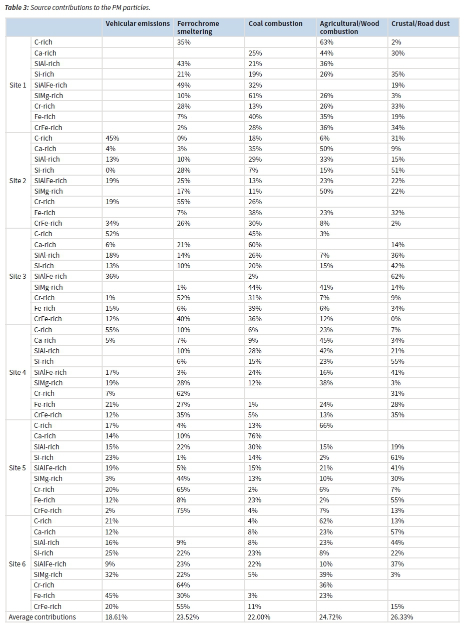
Source contributions to PM

PMF analysis determines the number of factors which correspond to potential particle sources. Source categories that potentially have contributed to ambient PM in the GTM rural area were identified as crustal/road dust, coal combustion fly ash, vehicle exhaust dust, agricultural/wood burning and industrial sources (Table 3). The average PM source contributions across all sites indicate that geological material (crustal/road dust) accounts for 26.33%. The crustal material could be mainly from resuspended dust from mine tailing in the area or transported from regional sources as indicated by the HYSPLIT transport pathways. Vehicular emissions are associated with tail pipe, emissions, tire and brake wear, road surface abrasion, wear and tear of other vehicle components such as the clutch, and resuspension of road surface dusts and accounted to 18.69% of the PM sources. Fly ash from industrial coal combustion contributed 22% to the PM in the study area. Most coal ash contain aluminium oxide (Al₂O₃), calcium oxide (CaO) and silicon dioxide (SiO₂) (Coal Ash, 2016). And regardless of the by-product produced, there are many toxic substances that are present in coal ash (such as arsenic, chromium, lead, mercury and uranium) that can cause major health problems in humans (Lockwood and Evans, 2016).

Agricultural and wood (cooking and space heating) burning accounts to 24.7% of the total PM emissions. The three ferrochrome smelters contributed 23.52% of the total PM in the airshed. The distribution of Cr elements across all source types indicate that ferrochrome smelters have a on the ambient air and have the potential to pollute the water bodies, which can impact on the human health since some of the communities in the area depend on water from the river streams for cooking and bathing.

Both PMF results and HYSPLIT clusters can be combined to make informed decisions on the sources and origin of PM sources. Crustal/road and soil dust can be transported by trajectories from both local and regional anthropogenic sources as shown in Fig. 1. However, it should be noted with caution that the trajectories are not accurately terrain following. Therefore, high-ending trajectories were chosen to represent more accurate boundary layer flow above the local terrain.

Emission reduction strategies

Source apportionment results can be useful for the review or development and implementation of strategies to reduce the impacts of pollution due to industrialization. Some of the immediate interventions to be considered in GTM are;

• Address fugitive emissions from industrial activities

• Review of the separation process of silica and chrome from milling process

• Review of the handling and transportation of milled chrome by road (as some of this material is spilled on the road)

• Effective enforcement of the Air Quality Act by authorities

• Reduction of fugitive emissions from smelters during material handling.

• Electrification of households to reduce wood burning.

• Reduction of dust from mine tailings and haul roads.

• Re-look at the transportation of ground milled chromium to address the current scourge of spillages on the roads.

• Initiate waste collection from rural households to prevent waste burning.

• These interventions can also be copied to other areas in South Africa.

 

Conclusion

The study investigated a selection of the chemical components of PM collected over a period of a year in the Greater Tubatse Municipality in Limpopo province of South Africa. The chemical components were used in PMF analysis for source profiling and source identification. HYSPLIT model was used in the identification of possible pollution source locations using backward clusters. The combination of the two models assisted in concluding that the sources can be either of local or regional origin.

These results show that the composition and levels of PM in GTM varied significantly among the six sites, however, systematic sampling and characterization of PM is needed in order to increase the sampling numbers and improve PMF results.

The PMF analysis identified a mixture of tracer elements as markers for source identification. However, differentiating these markers for different sources in the area has proved to be very difficult. This is because some of the chemical components that are solely industrial can find their way into other source categories such soil and road dust through deposition, and wood and agricultural plantation through absorption from the soil. The average source contributions were dominated by crustal/road dust, industrial activities such as ferrochrome smelters, and wood burning for space heating, with industrial coal burning, agricultural activities and vehicle emissions being other sources identified in the area. The contribution of this sources varied across the study area with chromium pollution being concentrated closer to the sources. These results show that the composition and levels of PM in GTM varied significantly among the six sites indicating the existence of varying microenvironments within the airshed, however, systematic sampling and characterization of PM is needed in order to increase the sampling numbers and improve PMF results.

This study can serve as a base for siting of AQ monitoring stations to ensure harmonized AQ assessments throughout the GTM. It can also be used as a guiding document for strengthening intervention strategies in the industrialized areas across South Africa.

 

Acknowledgements

The author acknowledges the South African Weather Service for financial assistance during the sampling period. RJ Lee for chemical analysis, NOAA Air Resources Laboratory for providing the HYSPLIT model and NOAA/OAR/ESRL PSD, Boulder, Colorado, USA for the NCEP Reanalysis data. The author also acknowledges Prof. Phillip Hopke from Clarkson University for his advice on the treatment of CCSEM results before application of PMF, and Dr. Thomas M Peters from University of Iowa for providing the formula for calculating single particle concentrations.

 

References

Ault A., Moore M., Furutani H., and Prather K. 2009. Impact of emissions from the Los Angeles port region on San Diego air quality during regional transport events, Environ. Sci. Technol., 43: 3500-3506.         [ Links ]

Barrera, V. A., Miranda, J., Espionosa, A. A., Meinguer, J. N., Ceron, E., Morales, J. R., Miranda, P. A., and Dias., J. F. 2012. Contribution of Soil, Sulfate, Biomass Burning Sources to the Elemental Composition of PM₁₀ from Mexico City. Int. J. Environ. Res., 6(3): 597-612.         [ Links ]

Begum, B.A., Kim, E., Biswas, S.K. and Hopke, P.K. 2004. Investigation of Sources of Atmospheric Aerosol at Urban and Semi-Urban Areas in Bangladesh. Atmos. Environ. 38: 3025-3038.         [ Links ]

Bhave, P.V., Fergenson, D.P., Prather, K.A. and Cass, G.R. 2001. Source Apportionment of Fine Particle Matter by Clustering Single-Particle Data: Tests of Receptor Model Accuracy. Environ. Sci. Technol. 35: 2060-2072.         [ Links ]

Buhot, A and W. Krauth. 1999. Phase separation in two dimensional additive mixtures. Phys. Rev. E 59: 2939-2941.         [ Links ]

Casuccio, G. S., Janocko, P. B., Lee, R. J., Kelly, J. F., Dattner, S. L., and Mgebroff, J. S. 1983a. The Use of Computer Controlled Scanning Electron Microscopy in Environmental Studies, J. Air Pollut. Control Assoc. 33:937.         [ Links ]

Central Pollution Control Board. Delhi, India (2010). Air quality monitoring, Emission Inventory and source apportionment study for Indian Cities - National Summary Report. http://moef.nic.in/downloads/public-information/Rpt-air-monitoring-17-01-2011.pdf        [ Links ]

Chen, W.N., Chen, Y.C., Kuo, C.Y., Chou, C.H., Cheng, C.H., Huang, C.C., Chang, S.Y., Ramana, M.R., Shang, W.L., Chuang, T.Y. and Liue, S.C. 2014. The real-time method of assessing the contribution of individual sources on visibility degradation in Taichung. Sci. Total Environ. 497-498: 219-228.         [ Links ]

Coal Ash: Characteristics, Management and Environmental Issues" (PDF). Electric Power Research Institute. Retrieved 3 March 2016.         [ Links ]

Community Empowerment Impact Assessment Report: Phase 1. 2007. https://www.nra.co.za/content/Tubatse1.pdf        [ Links ]

Dockery DW. 2001. Epidemiologic evidence of cardiovascular effects of particulate air pollution. Environ. Health Perspect. 109(4): 483-486.         [ Links ]

Draxler, R. R. and G. D. Hess, 1997: Description of HYSPLIT_4 modelling system. NOAA technical memorandum ERL ARL-224: 24pp.         [ Links ]

Draxler, R. R. and G. D. Hess, 1998: An overview of the HYSPLIT_4 modelling system for trajectories, dispersion and deposition. Australian Meteorological Magazine, 47: 295-308.         [ Links ]

Draxler, R., Stunder, B., Rolph, G., and Stein, A. 2018. HYSPLIT4 USER's GUIDE. Version 4. NOAA Air Resources Laboratory.         [ Links ]

European Commission. 2014. European Guide on with Receptor Models Air Pollution Source Apportionment. doi: 10.2788/9307.         [ Links ]

Goovaerts, P. 1997. Kriging vs stochastic simulation for risk analysis in soil contamination. In: Soares, A., Gomez-Hernandez J., Froidevaux R. (Eds.), geo-ENV I - Geostatistics for Environmental Applications. Kluwer Academic Publishers, Dordrecht, 247-258.         [ Links ]

DWAF, 2005. Water Services Planning Reference Framework, Sekhukhune District Municipality. DWAF, Enviromap and GPM Consultants, Pretoria, 124pp.         [ Links ]

Harris, A.R. and Davidson, C.I. 2005. The Role of Resuspended Soil in Lead Flows in the California South Coast Air Basin. Environ. Sci. Technol. 39: 7410-7415.         [ Links ]

Hockaday, S. and Bisaka, K. 2010. Some Aspects of the Production of Ferrochrome Alloys in Pilot DC Arc Furnaces At. In: The Twelfth International Ferroalloys Congress. 367-376.         [ Links ]

Hopke, P.K., and Casuccio, G. 1991. Scanning Electron Microscopy. In: Receptor Modeling for Air Quality Management. Elsevier, p. 7.         [ Links ]

Karanasiou A., Minguillόn M. C., Viana M., Alastuey A., Putaud J. P., Maenhaut W., Panteliads P., Močnik G., Favez O., and Kuhlbusch T. A.J. 2015. Thermal-optical analysis for the measurement of elemental carbon (EC) and organic carbon (OC) in ambient air: a literature review. Amos. Meas. Tech. Discuss., 8: 9649-9712.         [ Links ]

Kim, D.S., Hopke, P.K., 1988. The classification of individual particles based on computer-controlled scanning electron microscopy data. Aerosol Sci. Technol. 9: 133-151.         [ Links ]

Kim, E., T.V. Larson, P.K. Hopke, C. Slaughter, L.E. Sheppardand Claiborne, C. 2003b. Source Identification of PM_2.5 in an Arid Northwest U.S. City by Positive Matrix Factorization. Atmos. Res. 66: 291-305.         [ Links ]

Kim, E. and Hopke, P. K. 2008: Source characterization of ambient fine particles at multiple sites in the Seattle area, Atmos. Environ., 42: 6047-6056.         [ Links ]

Lagudu U.R.K, Raja S, Hopke P.K, Chalupa D.C, Utell M.J, Casuccio G, Lersch T.L, and West R.R., 2011. Heterogeneity of Coarse Particles in an Urban Area. Environ. Sci. Technol. 45: 3288-3296.         [ Links ]

Lee, E., Chan, C.K., Paatero, P., 1999. Application of positive matrix factorization in source apportionment of particulate pollutants in Hong Kong. Atmos. Environ. 33 (19): 3201- 3212.         [ Links ]

Liu, Y., Zhang W., Yang W., Bai Z., and Zhao X., 2018. Chemical Compositions of PM_2.5 Emitted from Diesel Trucks and Construction Equipment. Aer. Sci. & Eng 2:51-60.         [ Links ]

Lockwood, A. H., and Evans, L. "How Breathing Coal Ash Is Hazardous To Your Health". Physicians for Social Responsibility. Retrieved 3 March 2016        [ Links ]

Mamane Y., Willis R., and Conner T., 2001. Evaluation of Computer-Controlled Scanning Electron 381 Microscopy Applied to an Ambient Urban Aerosol Sample. Aerosol Science and Technology: The 382 Journ. Amer. Ass. Aer. Res., 34(1): 97.         [ Links ]

Moody, J. L. and Galloway, J. N. 1988. Quantifying the relationship between atmospheric transport and the chemical composition of precipitation on Bermuda. Tellus 40B, 463-479.         [ Links ]

Nkohla, M.A., 2006. Characterization of Ferrochrome Smelter Slag and its Implications in Metal Accounting, Cape Peninsula University of Technology, Cape Town, South Africa. 1-10.         [ Links ]

Ott, D. K., Cyrs, W, and Peters T.M. 2008. "Passive Measurement of Coarse Particulate Matter, PM₁₀-2.5." J. of Aeros. Sc. 39 (2): 156-167.         [ Links ]

Pant P. and Harrison R. M. 2012. Critical review of receptor modelling for particulate matter: A case study of India. Atmos. Environ. 49: 1-12.         [ Links ]

Pope CA III. 2000. What do epidemiologic findings tell us about health effects of environmental aerosols? Aerosol Med. 13(4):335-354.         [ Links ]

Ravindra, K., Bencs, L., Wauters, E., de Hoog, J., Deutsch, F., Roekens, E., Bleux, N., Bergmans, P. and Van Grieken, R. 2001. Seasonal and site specific variation in vapor and aerosol phase PAHs over Flanders (Belgium) and their relation with anthropogenic activities. Atmos. Environ, 40: 771-785.         [ Links ]

Reff, A., Eberly, S. I., and Bhave, P. V. 2007. Receptor modeling of ambient particulate matter data using positive matrix factorization: review of existing methods. JAPCA J. Air Waste Manag. 57: 146-154.         [ Links ]

Romesburg, H. C. 1984: Cluster analysis for researchers. Lifetime Learning, Belmont, Calif., 334pp.         [ Links ]

Sawvel, E.J., Willis, R., West, R.R., Casuccio, G.S., Norris, G., Kumar, N., Hammond, D., and Peters T.M. 2015. Passive sampling to capture the spatial variability of coarse particles by composition in Cleveland, OH. Atmos. Environ., 105: 61-69.         [ Links ]

Schauer, J.J., W.F. Rogge, L.M. Hildemann, M.A. Mazurek, G. R. Cass, and B.R.T. Simoneit. 1996. Source apportionment of airborne particulate matter using organic compounds as tracers. Atmos. Environ. 30:3837-55. doi:10.1016/1352-2310(96)00085-4.         [ Links ]

Schulze B. R. 1986. Climate of South Africa. Part 8. General Survey, WB 28, Weather Bureau, Department of Transport, Pretoria, 330 pp.         [ Links ]

Song, X.H., Hopke, P.K., 1996b. Solving the chemical mass balance problem using an artificial neural network. Environ. Sci. Technol. 30 (2): 531-535.         [ Links ]

Stohl, A. 1998. Computation, accuracy and applications of trajectories - a review and bibliography, Atmos. Environ., 32: 947-966.         [ Links ]

Stunder, B. J. B. 1996. An assessment of the quality of forecast trajectories. J. of Appl. Meteor. 35: 1319-1331.         [ Links ]

Sun H, Shamy M, Kluz T. 2012. Gene expression profiling and pathway analysis of human bronchial epithelial cells exposed to airborne particulate matter collected from Saudi Arabia. Toxicol. Appl. Pharmacol. 265:147-57.         [ Links ]

UNEP, 2006. African Regional Implementation Review for the 14th Session of the Commission on Sustainable Development.         [ Links ]

Van Groenigen, J.W., Stein, A. and Zuurbier, R. 1997. Optimization of environmental sampling using Interactive GIS. Soil Technology 10: 83-97.         [ Links ]

Wagner, Jeff, and David Leith. 2001b. "Passive Aerosol Sampler. Part II: Wind Tunnel Experiments." Aeros. Sc. & Tech. 34 (2): 193-201.         [ Links ]

Watson, J.G. and Chow, J.C. 2001a. PM_2.5 Chemical Source Profiles for Vehicular Exhaust, Vegetation Burning, Geological Materials and Coal Burning in Northwestern Colorado during 1995. Chemosphere. 43: 1141-1151.         [ Links ]

Watson, J.G. and Chow, J.C. 2001b. Source Characterization of Major Emission Source in the Imperial and Maxicali Valleys along the US/Mexico Boarder. Sci. Total Environ. 276: 33-47.         [ Links ]

Watson, J.G. 2002. Visibility: science and regulation. J. of Air and Waste Manag. Ass. 52: 628-713.         [ Links ]

Zayed A.M and Terry M., 2003. Chromium in the environment: factors affecting biological remediation. Plant and Soil 249: 139-156.         [ Links ]

 

 

† Deceased on 7 November 2017[R1]

 

 

Appendix A:

 

Figure A1 - Click to enlarge

 

 

 

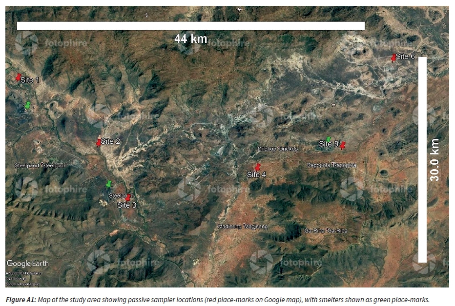
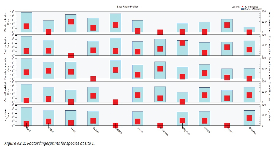
Figure A2.1 - Click to enlarge

 

 

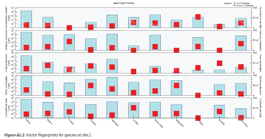
Figure A2.2 - Click to enlarge

 

 

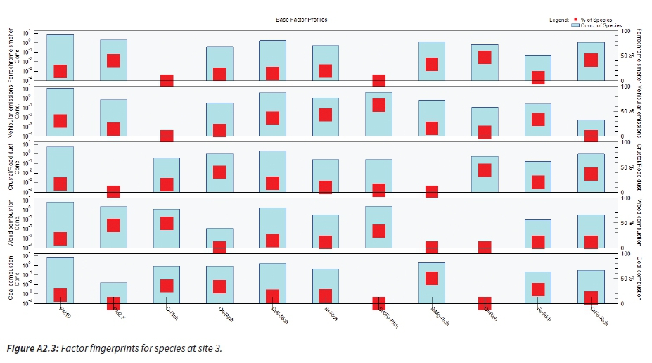
Figure A2.3 - Click to enlarge

 

 

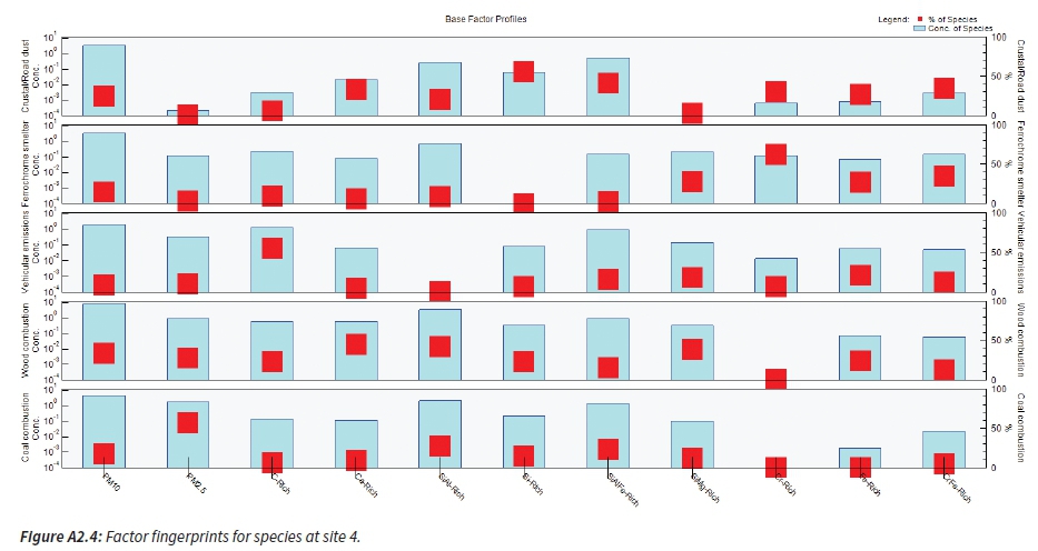
Figure A2.4 - Click to enlarge

 

 

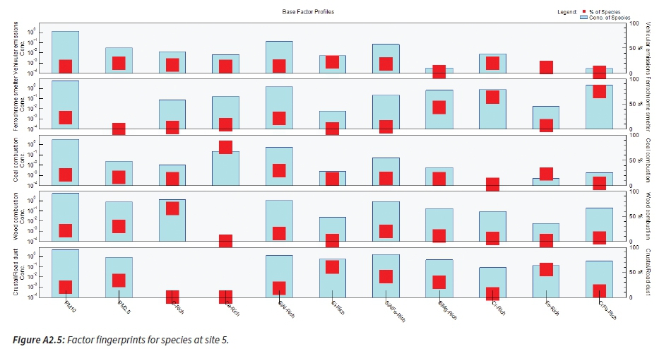
Figure A2.5 - Click to enlarge

 

 

Figure A2.6 - Click to enlarge