RESEARCH ARTICLE

 

Ht-index for empirical evaluation of the sampled graph-based Discrete Pulse Transform

 

 

Mark de Lancey; Inger Fabris-Rotelli

Department of Statistics, University of Pretoria, South Africa. Email: Mark de Lancey mark.stephen.del@gmail.com (corresponding), Inger Fabris-Rotelli inger.fabris-rotelli@up.ac.za

 

 

---

ABSTRACT

The Discrete Pulse Transform (DPT) makes use of LULU smoothing to decompose a signal into block pulses. The most recent and effective implementation of the DPT is an algorithm called the Roadmaker's Pavage, which uses a graph-based algorithm that produces a hierarchical tree of pulses as its final output, shown to have important applications in artificial intelligence and pattern recognition. Even though the Roadmaker's Pavage is an efficient implementation, the theoretical structure of the DPT results in a slow, deterministic algorithm. This paper examines the use of the spectral domain of graphs and designing graph filter banks to downsample the algorithm. We investigate the extent to which this speeds up the algorithm and allows parallel processing. Converting graph signals to the spectral domain can also be a costly overhead, so methods of estimation for filter banks are examined, as well as the design of a good filter bank that may be reused without needing recalculation. The sampled version requires different hyperparameters in order to reconstruct the same textures of the image as the original algorithm, selected previously either through trial and error (subjective) or grid search (costly) which prevented studying the results on many images effectively. Here an objective and efficient way of deriving similar results between the original Roadmaker's Pavage and our proposed Filtered Roadmaker's Pavage is provided. The method makes use of the Ht-index which separates the distribution of information in the graph at scale intervals by recursively calculating averages on decreasing subsections of the scale data stored. This has enabled empirical research using benchmark datasets providing improved results. The results of these empirical tests showed that using the Filtered Roadmaker's Pavage algorithm consistently runs faster, using less computational resources, while having a positive SSIM (structural similarity) with low variance. This provides an informative and faster approximation to the nonlinear DPT, a property which is not standardly achieveable.
CATEGORIES: • Mathematics of Computing ~ Probability and Statistics • Probability and Statistics ~ Probabilistics Algorithms

Keywords: Discrete Pulse Transform, graph sampling, multiscale, Ht-index

---

 

 

1 INTRODUCTION

The Discrete Pulse Transform (DPT) decomposes a signal into block pulses using LULU smoothers in such a way that the signal can be reconstructed fully (Fabris-Rotelli & Anguelov, 2010). The LULU smoothers L_kand U_kare applied recursively from k = 1 to K to obtain the DPT, the sequential decomposition of a signal f (such as an image) into scale levels Di(f ), D₂(f ), D₃(f), D_K(f) such that the sum of these gives the original signal f = ^K=i D_k(f ). Each scale level consists of block pulses (connected components) of size k.

This in turn has been used to detect features in signals and extract textures from images by partial reconstruction of the pulses. Feature and texture extraction has important applications in artificial intelligence, pattern recognition and computer vision (Laurie & Rohwer, 2007). Applying LULU operators directly on a signal using first principles until the signal is fully decomposed results in an operation of O(N³) complexity (Laurie, 2010). To create a more feasible implementation, a graph based algorithm known as the Roadmaker's algorithm was developed, which reduced the computational complexity to O(N) (Laurie & Rohwer, 2006). The main shortfall of the Roadmaker's algorithm is that its storage of block pulses requires a hierarchical tree containing sparse matrices at each node, which makes extraction of the pulses (and therefore reconstruction of the image) slow as well as storage requirements of the data structure relatively high. An improvement on this comes in the form of the Roadmaker's Pavage algorithm (Stoltz, 2014). This algorithm is also a graph based implementation, however the final data structure produced does not require sparse matrix storage at each node. The decomposition stage of the Roadmaker's Pavage is still O(N) and does not give an improvement on decomposition time, its advantage comes in the form of an improved resulting data structure that requires significantly less storage as well as a faster reconstruction and access time.

It should be noted that although the implementation algorithms of the DPT have reduced to linear complexity, the algorithms are still computationally slow. This is due to the algorithms needing to be processed in series, as well as the comparisons and transformations of data structures required at each step. Hence the true computational times needed is somewhat masked by the Big-O complexity. There is still a need to reduce to computational time, particularly for real-time application. The fact that these newer implementations are in the form of graph structures provides several advantages, especially considering the recent advances in theory and application of graph sampling and interpolation methods.

The research conducted here makes use of such recent developments in graph sampling and graph spectral theory to improve the running time and memory requirements of the Road-maker's Pavage algorithm by using an approximation of the algorithm and its output. In addition to this, any advantages that come with graph spectral analysis is now also introduced to the algorithm. The primary mechanism behind these improvements comes from the use of graph spectral filters and graph sampling methods. This is the first approximation algorithm for the DPT and it makes use of graph filtering. The DPT is a unique multi-scale decomposition and does not have a similar technique to be compared to. However, graph representation of images is a relevant topic, see Shekkizhar and Ortega (2020) for example, as well as efficiency in graph neural networks (Scarselli et al., 2009; Wu et al., 2020).

Appropriate scales of the multi-scale DPT decomposition are selected using the Ht-index developed by Jiang (see for example Jiang and Junjun (2013)). The Ht-index is an alternative fractal measure more appropriate for images and other spatial data. It has been shown to be useful in image content separation (Fabris-Rotelli & Stein, 2020). This provides a further improvement in the algorithm in a data-driven approach to selecting scales.

The paper begins with an overview of the suggested algorithm and its components in Section 2, and then demonstrates application of the algorithm in Section 3, before concluding in Section 4.

 

2 METHODOLOGY

The method used to improve computational speed of the Roadmaker's Pavage algorithm involves the use of a graph spectral filter bank. The reason behind filtering the signals is in order to band limit the signal. Band limited graph signals can be interpolated with perfect reconstruction after sampling under certain conditions (Siheng et al., 2015). The graph filter bank used makes use of two filters (low-pass and high-pass) to split the original image into its low and high frequency components. The high and low frequency signals are then passed on to each pipeline of the bank at which point each signal is operated on independently of the other. The remaining operations after filtering include:

1. Downsampling the filtered signals

2. Performing the DPT decomposition using Roadmaker's Pavage on the filtered signals

3. Full or partial reconstruction of the pulses stored within the tree structure

4. Upsampling the reconstructed signal

5. Filtering again the upsampled signals

6. Summing the signals and multiplying them with a constant to obtain the final output signal.

Hence the algorithm results in two smaller trees containing low frequency and high frequency pulses. After reconstruction of the desired pulses the signals produced are then upsampled, filtered again and combined together to obtain the final output signal. Each filter and pipeline operates completely independent from the other, and extraction of pulses from either tree is independent from each other. Because of this, the new algorithm has become what is known as embarrassingly parallel, that is, the job of parallel processing the filter bank and signals is trivial as the only time the two independent pipelines need to communicate with each other is at the very end where the two output signals are added together. The Roadmaker's Pavage wedged between filter banks is shown in Figure 1. The individual components of the filter bank and algorithm are explained next.

2.1 Roadmaker's Pavage decomposition and extraction DPT_dcand DPT_ex

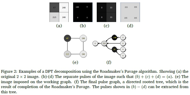
The Roadmaker's Pavage is a graph-based algorithm that results in a tree that contains the information required to extract the same pulses as defined by the DPT. The algorithm starts by imposing the image on a rectangular grid graph, known in this context as the Working Graph. Through a series of edge contractions, comparisons and clusterings, this Working Graph is eventually transformed into a tree. An example of the pulses extracted from a small 2 x 2 image, as well as the data structures built by the Roadmaker's Pavage is shown in Figure 2.

The Working Graph that is initialised is an example of a rectangular grid graph, which is also a bipartite graph. Even though the final product of the Roadmaker's Pavage is a tree, the extracted pulses need to be reshaped into an image with the same dimensions as the original in order to be meaningful. The reshaped output signal is not contained in a graph, but its properties and relations still behave as if it was imposed a new grid graph with the same dimensions as the original working graph. Thus, filtering, sampling and interpolation is based on this Working Graph structure. The original signal is on a graph of this type and is filtered and sampled from accordingly, while the output signal is upsampled and filtered as if it were a signal on a new grid graph. For these reasons the Roadmaker's Pavage decomposition, as well as extraction of the desired pulses, is inserted into the middle of the filter bank.

2.2 Graph Spectral Filters H₀(A) and Hi (A)

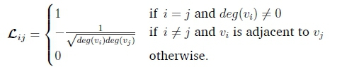
H₀ (A) and Hi (A) are low and high pass filters respectively. They first convert a graph signal, x e R^N with each x_idefined on vertex i, into its graph spectral domain using the Graph Fourier Transform (GFT). The signal is then converted back to the vertex domain using the Inverse Graph Fourier Transform (IGFT). The Graph Fourier Transform can be obtained from the eigendecomposition of a graph shift operator (Cheung et al., 2018; Narang & Ortega, 2012; Sakiyama et al., 2019; Siheng et al., 2015; Tremblay et al., 2018). An example of a graph shift operator is the adjacency matrix, A e R^NxNwhere = Aji = 1 if i = j and v_iis adjacent to v_jotherwise Aj = 0 (for undirected, unweighted graphs).

An alternative shift operator derived from A is the Laplacian Matrix, L (Cheung et al., 2018; Narang & Ortega, 2012; Sakiyama et al., 2019; Shuman et al., 2011; Tremblay et al., 2018). This is the difference of a graph's degree matrix D (whose diagonal entries gives the number of edges protruding from the corresponding node) and its adjacency matrix. Hence the Laplacian is defined by L = D - A. Finally, the most important shift operator to be used in this paper is the symmetric normalised Laplacian, L (Narang & Ortega, 2012; Sakiyama et al., 2019). The symmetric normalised Laplacian is given by L = DLD = I - D AD, with:

As the name implies, this version of the Laplacian is always symmetric, hence its eigenvector basis is real and orthogonal (Narang & Ortega, 2012; Tremblay et al., 2018). Some other important properties of the symmetric normalised Laplacian in the spectral domain include the fact that its eigenvalues range from 0 to 2 (Narang & Ortega, 2012; Tremblay et al., 2018) and since the graph used in the Roadmaker's Pavage is bipartite (described in section 2.4) its eigenvalues are also symmetric around 1. Now that L has been defined, its eigendecomposition is given by

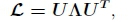
where A is a diagonal matrix containing the eigenvalues [X_i, X₂,X_N} of L and the columns of U contains the eigenvectors of L . This eigenbasis is orthonormal, hence U^-1= U^T.

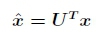
Definition 1. The Graph Fourier Transform is the projection of a graph's signal in its vertex domain to the graph's spectral domain. For a diagonalisable graph shift operator L = UAU^T on graph G, the Graph Fourier Transform of graph signal x e R^N is given by:

Alternatively it may be defined by its evaluation at each eigenvalue:

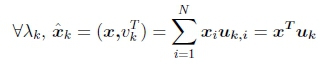
where u_k is the eigenvector associated with the k^th eigenvalue of L, which is also the k^th column of U (Cheung et al., 2018; Sakiyama et al., 2019; Tremblay et al., 2018).

The GFT is invertible, as UX =UU^-1x = x. With the GFT defined, graph spectral filters can be constructed.

Definition 2. A Graph Spectral Filter is a function that projects separately on each of the eigenspaces of L depending on the value of the respective X. Mathematically, a kernel X - h(X), defines a graph filter H such that H = U h(A)U^T.

Hence a filtered signal is defined such that x_h = Hx. Several kernels are suitable to define a filter. The simplest is to use an indicator function that cuts off certain frequencies completely, such as h(X) = 1 if X < w, else h(X) = 0, where w is the desired cut-off frequency. The filter used here is a graph quadrature mirror filter (graph-QMF) so that:

1. H₀and H_iare used in both the analysis and synthesis bank of each respective pipeline, as opposed to different filters used at each end,

2. H₀ = H_i(2 - X). Recall that the eigenvectors of L are symmetric around 1 and range from 0 to 2, and

3. Ho²(X) + H²(X) = c²

where 1/c² is a constant that scales the final output signal (Narang & Ortega, 2012). For a simple indicator kernel where w = 1, c²= 2.

Finally, of note is the fact that exact calculation of these graph filters requires calculation of the full eigenspectrum as well as the dense eigenvector matrix U of size N² which can require more memory space than available for large N. For this reason, Chebyshev polynomials are used to approximate the response of x_h = Uh(A)U^Tx. This is because h(X) can be approximated as a Kth order polynomial (Shuman et al., 2011).

2.3 Scale Selection

In Fabris-Rotelli and Stein (2020) it is shown that the Ht-index is suitable for identifying structure locations within the scales of the Discrete Pulse Transform. The Ht-index is the number of repetitions required to obtain the mean-scale as a threshold with the majority (taken as more than 50%) of scale objects to the left. The full DPT provides a distribution of pulses at each scale, with the distribution being heavily skewed to the right, with the vast majority of pulses being of smaller scales. Once this distribution has been obtained by inspecting the output pulse graph structure, the Ht-index can be found. This is done by repeatedly applying a mean to the scale distribution, as per the following procedure:

1. Find the mean scale of the pulses, mean!.

2. Determine the number of pulses that are smaller than this mean (n_less), and larger than this mean (n_more).

3. If n_less > n_more, repeat this procedure on the pulses to the right of this mean, the tail.

The Ht-index is determined as one plus the number of times step 2 is true. We discuss a short example to explain the calculation of the Ht-index. Consider data which has a number of structures at the following scale (1,2,3,4,5,6,7) with the number of structures at each of these scales beings (5000,4000,3000,1000,500,100,1) respectively. The mean scale is calculate as

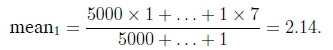
The number of structures larger than meani is 3000 + ... + 1 = 4601 = n_more and the number of structures smaller than mean₁ is 5000 + 4000 = 9000 = n_less. Since n_less> n_more we repeat this procedure on the tail (3,4,5,6,7), calculating mean₂ = 3.5. Using mean₂ on the tail scales, n_more = 1601 and n_less = 3000. Once again n_less> n_more so we repeat this procedure on the tail (4,5,6,7), calculating mean₃ = 4.44. Using mean₃ on the new reduced tail scales, n_more = 691 and n_less = 1000. Once again n_less> n_more so we repeat this procedure on the tail (5,6,7), calculating mean₄ = 5.17, n_less = 500 and n_more = 201. We repeat once again on tail (6,7), calculating mean₅ = 6.01, n_less = 100 and n_more = 1. This toy example thus has an Ht-index of 6. The scale intervals are the scales to the left of the mean at each repetition. In real images the scales are more meaningful than this simple example, providing objective breaks in the scale distribution. In Fabris-Rotelli and Stein (2020), these scale intervals are used to reduce a big data context to the scale intervals containing the information of the image. This concept is made use of here.

Previously, in de Lancey and Fabris-Rotelli (2019), relatively subjective methods were used to select scales to compare images. Scales were selected by altering the scale bracket until a certain similarity was noted visually and then could be verified using MSE or SSIM. Alternatively a grid-search yielded the most similar two images after finding the best selection of scales from all possible combinations but this was found to have prohibitive computational costs. The use of the Ht-index in Fabris-Rotelli and Stein (2020) provides a new heuristic that was found to be both computationally efficient and provided similar images. Another advantage of using the Ht-index is that it selects the result a priori to validation (unlike using the grid search) as it is based solely on the distribution of the structures being measured, as opposed to making use of a compared MSE to find a suitable image.

2.4 Upsampling and downsampling operators l S and t S

The operators S_d0, S_di and S_u0,S_ulare used to downsample and upsample signals, respectively. Downsampling is done by simply taking only the n < N vertices and corresponding signals in the graph that are chosen so that R^N - Rⁿ. Upsampling increases the dimension of a sampled signal to the original graph dimensions, imposing the signal on the original vertices and then fills any missing values with zeroes. The initial graph used in the Roadmaker's Pavage algorithm is a grid graph, which is also a bipartite graph. A bipartite graph is a graph that can be divided into two disjoint and independent sets V_Bottomand V_Topsuch that every edge connects a vertex in V_Bott_omto one in V_Top, while the vertices within a set are not connected to each other. Sampling a bipartite graph signal according to these disjoint bipartite sets is a standard procedure when sampling is required, as the sets will cover a large area of the graph with approximately equal spacing between both sampled and excluded vertices. This makes interpolation of an upsampled signal more accurate as each empty excluded node will have several neighbours used to interpolate its value (Narang & Ortega, 2012; Sakiyama et al., 2019).

There is however, a major caveat when using bipartite sampling for the Roadmaker's Pavage. By definition, each bipartite set has no connections within itself but the Roadmaker's Pavage requires a connected graph in order to perform the required transform and comparisons. To remedy this, an adjusted graph is used for sampling. First, vertex indices to be sampled are chosen in a bipartite manner as usual. Additional diagonal edges are then used to join nodes together. Finally the two sets are separated from each other as if the graph is still bipartite, but now each set is connected. Thus the Roadmaker's Pavage algorithm can proceed on these sampled graphs. An example of this procedure performed on a small graph with 4 nodes is shown in Figure 3.

 

3 APPLICATION

In this section comparisons are made between the original Roadmakers Pavage algorithm and the proposed Roadmaker's Pavage used in conjunction with a filter bank. First, a more subjective but illustrative example is shown using an image of Chelsea the cat. Afterwards, by selecting scales using the Ht-index (described in Section 2.3), results of a simulation are shown that produce more objective results. This is done with a more meaningful and mathematically derived scale selection algorithm via the Ht-index approach of Fabris-Rotelli and Stein (2020).

The original image was decomposed into pulses using both methods. In the case of the sampled and filtered algorithm, it was found that the entire high frequency pipeline could be discarded for the cost of a small decrease in mean-squared-error and extraction accuracy of smaller features. This meant that only one line of filters and samplers was required in this instance as well as only a single tree data structure.

The image was then reconstructed both fully and partially in both cases. Partial reconstruction included extraction of only the smallest textures in the image, extraction of a mid-range of pulse sizes giving a smoothed image and extraction of the largest pulses giving the large features present in the image. The full and partial reconstruction of the image can be seen in Figure 4 while the equivalent reconstructions can be seen in Figure 5.

The machine used to test these applications had an Intel Core i7-7700HQ CPU running at 2.8 GHz (HQ means a quad core optimised for mobility and high performance). The RAM on this machine was 16GB. The operating system installed was Windows 10 Professional at 64 Bits. The same hardware and software was used for all trials. The system was rebooted and reset between each trial to ensure previous trials did not bias future ones. The hardware was never strained (e.g. CPU usage never at 100% and RAM never full) to ensure that hardware restrictions did not bias algorithm performance.

The original image has 135 300 pixels. The root-mean-squared-error between the fully reconstructed original image and the interpolated fully reconstructed image from the filtered Roadmaker's Pavage was 1.47. The original algorithm has an RMSE of zero as it perfectly reconstructs the original image. The error introduced by the filtered algorithm can be justified by the noticeable decrease in computational time and storage requirements. The original algorithm required 87 CPU seconds to decompose, approximately 5.5 CPU seconds to reconstruct the signals and needed a tree with 170 777 nodes to store the information. The filtered algorithm needed only 27.5 CPU seconds to decompose the signal, approximately 2.5 CPU seconds to reconstruct and a tree with 89 234 nodes for storage. A summary of these findings is given in Table 1.

For a more objective second method, a simulation along with scale selection methods and SSIM measurement were used. The SSIM has proven to be a useful image comparison tool (Sara et al., 2019). In order to do this, the Berkeley Segmentation Dataset and Benchmark (BSD 300) dataset¹ is used to test and compare both the original DPT and the new filtered algorithm. For each image in this dataset, the image is sent to both the original DPT and the Filtered DPT algorithms. Each algorithm then performs its decomposition stage independently of the other. Once the decomposition stage is complete, scale intervals are selected using the Ht-index. The first 3 intervals are selected from the original decomposition, as well as the first 3 intervals of both the low filtered decomposition and high filtered decomposition. Notably, some images of the database are too simple and had less than 3 scale intervals after being processed in one or more of the algorithms². These images were left out of the final comparison and only valid images with 3 intervals were used. This resulted in a final sample size of 253 of the 300 images in the database. Once these scale intervals were obtained, each valid image is reconstructed 3 times per algorithm (for each of the first three scale intervals). Filtered reconstructions are summed for each interval. Then for each of these Ht-Index defined partial reconstructions, the results were recorded. These results included the SSIM (structural similarity) (Z et al., 2004), an index related to the MSE, between the image reconstructed by the original algorithm and by the filtered algorithm, as well as CPU time, to see if there is a increase in efficiency by using the filtered algorithm.

These results are shown in Figures 6 to 9. In Figure 6 the distribution of the Ht-index is shown. The Ht-index gives an indication of the complexity of the image, with a larger index indicating the presence of more intricate textures within the image. It is therefore an expected result that the Ht-index for scale distributions found after low-pass filtering are on average simpler than those in the original image (as a low-pass filter behaves as a form of smoothing or simplification of an image). Figure 7 shows the distributions of CPU-times for the reconstruction phase of the simulations. This statistic highlights the entire purpose of this algorithm, as without a reduction of computation resources, this approximation algorithm of the DPT would serve no purpose. In comparison to the original Roadmakers Pavage algorithm, the filtered algorithm uses far less computational time. The low-frequency pipeline of the algorithm uses even less time that the high-frequency pipeline. This is to be expected once again due to the smoothing nature of a low-pass filter. The second boxplot of Figure 7 shows the fraction of CPU time required for decomposition, showing that most decompositions take less than half the time when compared with the original algorithm. Figure 8 shows reconstruction times for each interval as selected by the calculated Ht-structure and index. Once again these results are consistent. Each partial reconstruction is much faster using the filtered algorithms. There are exceptions for high-frequency reconstructions of the third interval, where some outliers take longer than the original algorithm. This can be explained by a more complex structure of high-frequency components resulting from images with complex textures. However, even in these scenarios there is considerable gain in efficiency when considering the average decomposition time, and reconstruction time for other intervals.

Figure 9 shows the SSIM index for original reconstructions and filtered algorithm reconstructions. The purpose behind this index in these simulations is to show that a certain level of similarity can be retained even after filtering and having a different structure and distribution of scales. The SSIM index ranges from -1, meaning that the images compared have no similarity, to 1 , indicating the images compared are identical. SSIM uses a set of tiles from each image being compared as a window.

The SSIM results here are from a very precise SSIM that used a tile-size of only 7 pixels. This in turn means that even small differences results in a highly penalised SSIM. Despite this very strict SSIM the filtered algorithm performed consistently well, having a positive SSIM for every image for each of the 3 fractals reconstructed.

The results presented are the first approximation algorithm for the DPT. Previous non-approximated implementations have not yielded any significant computational improvement. The construction of the Roadmaker's Pavage in Fabris-Rotelli and Stoltz (2012) introduced an improved storage of the extracted DPT resulting in better availability of the content for post-analysis but no significant algorithmic improvement. This paper provides the first algorithmic improvement to the original Roadmaker's algorithm of Laurie and Rohwer (2006).

 

4 CONCLUSION

This paper has shown that an approximation of the Discrete Pulse Transform can be obtained using the Roadmaker's Pavage algorithm in conjunction with graph spectral filtering and sampling, a notable achievement for a nonlinear operation. A minor loss of accuracy comes with the benefits of noticeably shorter computational time and storage requirements. Depending on the level of precision required and the size of the features needed, the high pass filters can be discarded if not necessary for the task. Even if the high frequencies are still needed, this approximate algorithm can now be calculated with two independent channels and thus can be parallel processed.

Simulations were conducted on the BSD300 dataset to find the distribution and consistency of these findings. Use of the Ht-Index and the SSIM allowed for an objective measure of accuracy and meaningful selections of reconstructions from images. Across different scale intervals as defined by the Ht-index structure, the new filtered algorithm performs well and consistently, having a positive SSIM with low variance. This sampling approach for the DPT should be further tested for accuracy in areas the DPT has been applied such as segmentation (Fabris-Rotelli & Greeff, 2012), feature detection (Fabris-Rotelli, 2011) and its effectiveness when considering leakage (Fabris-Rotelli & Stoltz, 2012).

 

ACKNOWLEDGEMENTS

This work is based upon research supported by the South Africa National Research Foundation and South Africa Medical Research Council (South Africa DST-NRF-SAMRC SARChI Research Chair in Biostatistics, Grant number 114613). Opinions expressed and conclusions arrived at are those of the author and are not necessarily to be attributed to the NRF.

 

References

Cheung, G., Magli, E., Tanaka, Y. & Ng, M. (2018). Graph spectral image processing. Proceedings of the IEEE, 106(5), 907-930. https://doi.org/10.1109/JPROC.2018.2799702        [ Links ]

de Lancey, M. & Fabris-Rotelli, I. (2019). Effective graph sampling of a nonlinear image transform. Proceedings of FAIR 2019, 2540, 185-195. http://ceur-ws.org/Vol-2540/        [ Links ]

Fabris-Rotelli, I. (2011). The Discrete Pulse Transform for images with entropy-based feature detection. In P. Robinson & A. Nel (Eds.), Proceedings of the 22nd Annual Symposium of the Pattern Recognition Association of South Africa 2011 (pp. 43-48). http://www.prasa.org/proceedings/2011/prasa2011-08.pdf

Fabris-Rotelli, I. & Anguelov, R. (2010). LULU operators and Discrete Pulse Transform for multidimensional arrays. IEEE Transactions on Image Processing, 19(11), 3012-3023. https://doi.org/10.1109/TIP.2010.2050639        [ Links ]

Fabris-Rotelli, I. & Greeff, J. (2012). The application of the iterated conditional modes to feature vectors of the Discrete Pulse Transform of images. In A. De Waal (Ed.), Proceedings of the 23nd Annual Symposium of the Pattern Recognition Association of South Africa 2012 (pp. 149-156). https://researchspace.csir.co.za/dspace/bitstream/handle/10204/6409/De%20Waal_2012.pdf?sequence=1#page=158

Fabris-Rotelli, I. & Stein, A. (2020). Use of fractals to measure anisotropy in point patterns extracted with the DPT of an image. Spatial Statistics, Accepted. https://doi.org/10.1016/j.spasta.2020.100452

Fabris-Rotelli, I. & Stoltz, G. (2012). On the leakage problem with the Discrete Pulse Transform decomposition. In A. De Waal (Ed.), Proceedings of the 23rd Annual Symposium of the Pattern Recognition Association of South Africa 2012 (pp. 179-186). http://researchspace.csir.co.za/dspace/bitstream/handle/10204/6409/De%20Waal_2012.pdf?sequence=1&isAllowed=y#page=188

Jiang, B. & Junjun, Y. (2013). Ht-index for quantifying the fractal or scaling structure of geographic features. Annals of the Association of American Geographers, 104. https://doi.org/10.1080/00045608.2013.834239        [ Links ]

Laurie, D. (2010). The roadmaker's algorithm for the Discrete Pulse Transform. IEEE Transactions on Image Processing, 20(2), 361-371. https://doi.org/10.1109/TIP.2010.2057255        [ Links ]

Laurie, D. & Rohwer, C. (2006). Fast implementationof the Discrete Pulse Transform. In G. Psihoyios, T. Simos & C. Tsitouras (Eds.), International conference ofnumerical analysis and applied mathematics 2006 (pp. 484-487).

Laurie, D. & Rohwer, C. (2007). The Discrete Pulse Transform. SIAM Journal on Mathematical Analysis, 38(3). https://doi.org/10.1137/040620862        [ Links ]

Narang, S. & Ortega, A. (2012). Perfect reconstruction two-channel wavelet filter banks for graph structured data. IEEE Transactions on Signal Processing, 60(6), 2786-2799. https://doi.org/10.1109/TSP.2012.2188718        [ Links ]

Sakiyama, A., Watanabe, K., Tanaka, Y. & Ortega, A. (2019). Two-channel critically sampled graph filter banks with spectral domain sampling. IEEE Transactions on Signal Processing, 67(6), 1447-1460. https://doi.org/10.1109/TSP.2019.2892033        [ Links ]

Sara, U., Akter, M. & Uddin, M. (2019). Image quality assessment through FSIM, SSIM, MSE and PSNR - comparative study. Journal ofComputer and Communications, 7(3), 8-18.         [ Links ]

Scarselli, F., Gori, M., Tsoi, A. C., Hagenbuchner, M. & Monfardini, G. (2009). The graph neural network model. IEEE Transactions on Neural Networks, 20(1), 61-80.         [ Links ]

Shekkizhar, S. & Ortega, A. (2020). Efficient graph construction for image representation. arXiv preprint arXiv:2002.06662.

Shuman, D., Vandergheynst, P. & Frossard, P. (2011). Chebyshev polynomial approximation for distributed signal processing. International Conference on Distributed Computing in Sensor Systems and Workshops (DCOSS) (2011). https://doi.org/10.1109/DCOSS.2011.5982158

Siheng, C., Varma, R., Sandryhaila, A. & Kovacevic, J. (2015). Discrete signal processing on graphs: Sampling theory. IEEE Transactions on Signal Processing, 63(24), 6510-6523. https://doi.org/10.1109/TSP.2015.2469645        [ Links ]

Stoltz, G. (2014). Roadmaker's pavage, pulse reformation framework and image segmentation in the Discrete Pulse Transform (Master's thesis). University of Pretoria. http://hdl.handle.net/2263/43255

Tremblay, N., Gonçalves, P. & Borgnat, P. (2018). Design of graph filters and filterbanks. Cooperative and graph signal processing (pp. 299-324). Academic press. https://doi.org/10.1016/B978-0-12-813677-5.00011-0

Wu, Z., Pan, S., Chen, F., Long, G., Zhang, C. & Philip, S. Y. (2020). A comprehensive survey on graph neural networks. IEEE Transactions on Neural Networks and Learning Systems.

Z, W., AC, B., HR, S. & EP, S. (2004). Image quality assessment: From error visibility to structural similarity. IEEE Transactions on Image Processing, 13(4), 600-612. https://doi.org/10.1109/TIP.2003.819861        [ Links ]

 

 

Received: 01 June 2020
Accepted: 30 September 2020
Available online: 08 December 2020

 

 

1 https://www2.eecs.berkeley.edu/Research/Projects/CS/vision/bsds/
2 Note that a larger Ht-index is indicative of larger complexity.