RESEARCH ARTICLE

 

Using Summary Layers to Probe Neural Network Behaviour

 

 

Marelie H. Davel

Multilingual Speech Technologies, North-West University, South Africa; and CAIR, South Africa. Email: Marelie H. Davel marelie.davel@nwu.ac.za

 

 

---

ABSTRACT

No framework exists that can explain and predict the generalisation ability of deep neural networks in general circumstances. In fact, this question has not been answered for some of the least complicated of neural network architectures: fully-connected feedforward networks with rectified linear activations and a limited number of hidden layers. For such an architecture, we show how adding a summary layer to the network makes it more amenable to analysis, and allows us to define the conditions that are required to guarantee that a set of samples will all be classified correctly. This process does not describe the generalisation behaviour of these networks, but produces a number of metrics that are useful for probing their learning and generalisation behaviour. We support the analytical conclusions with empirical results, both to confirm that the mathematical guarantees hold in practice, and to demonstrate the use of the analysis process.
CATEGORIES: • Computing methodologies ~ Neural networks • Theory of computation ~ Machine learning theory

Keywords: deep learning, machine learning, learning theory, generalisation

---

 

 

1 INTRODUCTION

Deep Neural Networks (DNNs) have been used to achieve excellent performance on many traditionally difficult machine learning tasks, especially high-dimensional classification tasks such as computer vision, speech recognition and machine translation (Goodfellow et al., 2016). DNNs generalise well: trained on a limited data set, they are able to transfer this learning to unseen inputs in a demonstrably effective way. Despite various approaches to studying this process (Bartlett et al., 2017; Dinh et al., 2017; Jiang et al., 2019; Kawaguchi et al., 2019; Keskar et al., 2017; Montavon et al., 2011; Neyshabur et al., 2017; Raghu et al., 2017; Shwartz-Ziv & Tishby, 2017), no framework yet exists that can explain and predict the generalisation ability of DNNs in general circumstances.

Specifically, one of the central tenets of statistical learning theory links model capacity- the complexity of the hypothesis space the model represents-with expected generalisation performance (Vapnik, 1989). However, a sufficiently large DNN represents an extremely large hypothesis space, specified by hundreds of thousands of trainable parameters. While any architecture that has a hypothesis space that is sufficiently large to be able to memorise random noise is not expected to generalise well, this is not the case for DNNs. In a paper that caused much controversy, Zhang et al. (2017) demonstrated how both Convolutional Neural Networks (CNNs) and standard Multilayer Perceptrons (MLPs) are able to memorise noise perfectly, while extracting the signal buried within the noise with the same efficiency as if the noise was not present. Even more pointedly, this was shown to occur with or without adding regularisation (Zhang et al., 2017).

The generalisation behaviour for even a straightforward fully-connected feedforward network - as soon as it has more than one layer and non-linear activation functions - has not yet been fully characterised In this work we take a step back, and analyse the classification ability of such a network with one change: we add a small 2-node summary layer to the more standard fully-connected feedforward network in order to be able to probe its behaviour during training and use.

In recent work (Davel et al., 2020), it was shown how the individual nodes of a standard fully-connected feedforward network can draw class-specific activation distributions apart, to the extent that these distributions can be used to train individual likelihood estimators and produce accurate classifications at any of the later layers of a network. Here we use these activation distributions to continue to probe the ability of a fully-connected feedforward network to generalise.

The main contribution of this paper is a conceptual analysis process that can be used to probe the generalisation ability of a neural network by adding a summary layer, and the empirical confirmation of the mathematical aspects of this analysis. In the process, we define the theoretical conditions for correct classification of a set of samples by an MLP, and use these conditions to analyse network behaviour. This paper is an extended version of (Davel, 2019), and repeats much of the preliminaries, in order to be readable on its own. Note that both the notation and derivation process have been made clearer, resulting in a different formalism for the theoretical conditions for correct classification. There has also been some shift in emphasis from focusing on gaps (differences in values) to ratios (relationships between values), as will become clearer in later sections.

In the next section, we start by reviewing the concept of nodes as network elements (Section 2), before introducing activation and weight ratios (Section 3), and exploring the role of these ratios in achieving perfect classification from an analytical perspective. Expected relationships are empirically confirmed in Section 4, before demonstrating the intention of the analysis process in Section 5.

 

2 NODES AS NETWORK ELEMENTS

While a network functions as a single construct, each layer also acts as a functional element, and within a layer, each node can be viewed as an individual unit with both a local and global function. Nodes are locally attuned to extracting information from a very specific part of the input space, while collaborating globally to solve the overall classification or regression task. Specifically, in Davel et al. (2020) it was shown that node-specific classifiers can be constructed from two different information sources: either utilising the continuous activation values (the distribution of activation values observed at a node), or the discrete counts of whether a node is active or not when presented with the training data. For all networks of sufficient size analysed, it was observed that at some layer, the network is able to achieve similar classification accuracy as the actual network, irrespective of the system used to perform classification (Davel et al., 2020).

This is an interesting result. In both systems, each node therefore uses locally available information to develop its own probability estimate in isolation, but then collaborates with other nodes (across the layer) to solve the overall classification task. Using this perspective, the set of samples that activates any node (its 'sample set') becomes very significant, as discussed further in Section 2.1.

We restrict the rest of this discussion to fully-connected feedforward architectures with rectified linear unit (ReLU) activations (Nair & Hinton, 2010) and arbitrary breadth (number of nodes in a hidden layer) and depth (number of hidden layers). Analysis is further restricted to solving a classification task, with stochastic gradient descent (SGD) to optimise network parameters.

2.1 Samplesets

Simultaneously introduced in Davel (2019) and Theunissen et al. (2019), a node-specific sample set refers to the set of samples that activates a specific node. During gradient descent, the forward process applies weights to create sample sets; the backward process uses sample sets to update weights: each weight attuned to its specific sample set. For ReLU-activated networks, this update has a surprisingly simple structure, if the weight update is written in its iterative form, as introduced in Davel et al. (2020), a derivation that we loosely follow here.

We define the sample set S_btij at node j of layer l as those samples in batch b that produce a positive activation value at node j. For any sample in the sample set, node j in layer l can be connected to an arbitrary number of active nodes in layer l + 1. Selecting one active node per layer, the weights connecting these active nodes can be used to define an active path p = {w_p1 ,w_p2,..., w_PN__l} associated with a specific sample, starting at layer l and ending at a node in the output layer N. Limiting our analysis to ReLU-activated networks with no bias values beyond the first layer, the SGD weight update ôw^j_icontribution from sample s, for the weight connecting node i in layer l - 1 to node j at layer l is then given by:

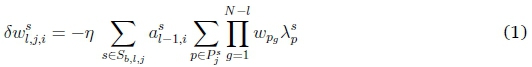
where the superscript s indicates sample-specific values, and

• n indicates the learning rate,

• a^s_l__1iindicates the post-activation value at node i in layer l - 1,

• P^findicates the set of all active paths linking node j to the output layer, and

• Xp indicates the derivative of an arbitrary loss function¹ with regard to the pre-activation value at node c_p; where c_pindicates the last node in path p, one of the possible output nodes, each associated with one of the possible classes.

This sample-specific weight update can be expressed in terms of the node-supported cost, a scalar value that represents the portion of the final cost that can be attributed to all active paths emanating from node j, when processing sample s. Specifically, the sample-specific node-supported cost (Cf,) at layer l, node j is defined as:

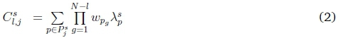
It is observable that C^f, does not differentiate between a node that creates paths with large positive and negative costs that balance out, and one where all individual paths have close to zero cost. Both have little effect on the specific weight update. Also, for a particular path p, a positive cost implies too much activation at the end node of that specific path, and a negative cost, too little.

The weight update calculate over all samples in the mini batch of size B is then given by:

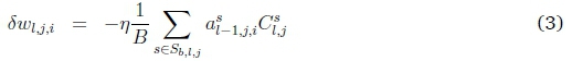
with the update to the node vector w_lj feeding into node j at layer l given by:

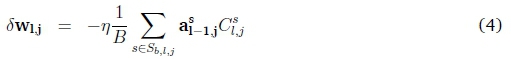
This sum can either be calculated over S_ltj, or over S_ltjn S_l__itias only samples that are active at both nodes i and j will contribute to the sum. The weight update is therefore directly specified by the batch-specific sample set, and only this sample set. Intuitively, it is produced by calculating the product of the activation value feeding into the node with the node-supported cost (per sample), summing these values over all samples in the cluster, and weighing this value with a constant. In Equation 3, both the local and global nature of the update is evident: the S_btij is a locally relevant set of samples, specific to this node; for each s e Sb,i,j, the cost C^fj is influenced by the state of the overall network, with the value representing a single node-specific summary of the sample's current error within the network.

 

3 GAPS AND RATIOS

In order to develop a theoretical perspective on the interplay between activation values, node-supported cost and sample sets, we introduce a summary layer to a standard MLP architecture. In this way, the summary layer provides a starting point for a theoretical analysis. This allows us to determine the exact theoretical requirements for perfect classification of a set of samples.

3.1 A simplified architecture

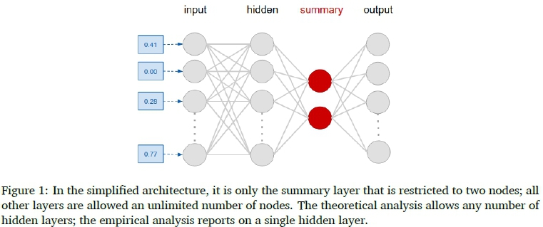
While an MLP is typically viewed as an input and output layer flanking any number of hidden layers, each hidden layer can also be seen as a small 3-layer subnetwork in its own right: utilising the output from the prior layer as input, and trying to address the loss (the node-supported cost of Section 2.1) passed along from its immediate output layer, the next hidden layer. As a starting point for our analysis, we consider a 3-layer subnetwork: considering only a single functional hidden layer in addition to an input and output layer. An additional hidden layer is now added between the functional hidden layer and the output as a summarising element: this layer contains only two nodes, in order to summarise the activations produced by the functional hidden layer for analysis purposes, as illustrated in Figure 1.

3.2 Theoretical requirements for perfect classification

Consider a network that only has two nodes in its last hidden layer. At least two nodes are required to be able to differentiate among classes, but two nodes are sufficient to differentiate among an unlimited number of classes, if weights are correctly assigned. From here onward, we omit the layer indicators, knowing we are only analysing activation values (a) at the summary layer, weight values (w) connecting the summary with the output layer, and the output values (z) at the final layer. Consider two samples s and t from two different classes c_sand c_t, respectively. Limit the nodes in the last hidden layer to two, arbitrarily named A and B, let a^s_Abe the activation value of sample s at node A, and w_CsAthe weight to the output node associated with class cs, starting at node A.

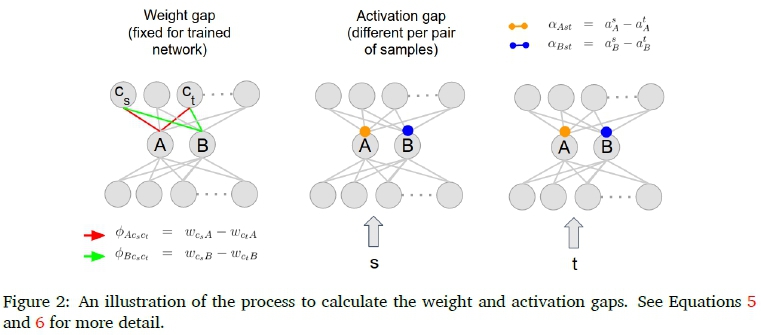
We can now define a number of values, the meaning of which will become clearer as this section progresses. The activation gap is defined as the difference between the activation values of two samples (s and t) at a node (A or B):

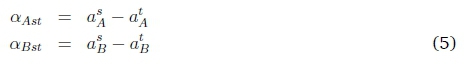
The weight gap 0 is defined as the difference between two weight values linking the same node to different nodes in the output layer:

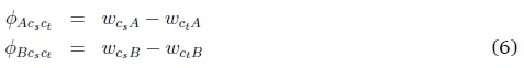
The weight gaps are not sample-specific, and have a single value for each summary node and pair of classes. They allow us to construct the first ratio we use in the analysis: the weight ratio. The weight ratio is defined as the ratio between the weight gaps of the two summary nodes:

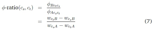
We will see later (in Equation 17) that this value is required to be positive for classification to be possible.

The activation ratio (a-ratio) is specific to each sample, and is defined as the ratio of the activation values between the two summary nodes:

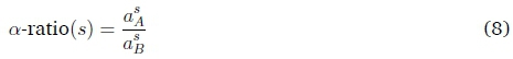
Note that, how A and B are used in the numerator and denominator is fixed and different for the two ratios. The choice is arbitrary, but remains fixed throughout the analysis. The definitions of weight and activation gaps are illustrated in Figure 2.

For a sample s to be classified correctly, we know that the sample-specific output value at z^s_Cashould be positive, and higher at node c_sthan at any other node. This is similar to requiring that, for any sample-pair s and t, it should hold that:

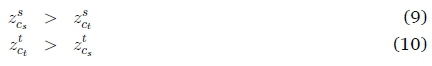
These requirements can be specified in terms of the newly defined weight and gap ratios. Specifically, consider a network with two summary nodes A and B and weights connecting each summary node to each of the output nodes (one per class), such that all weights from a single summary node are distinct, that is:

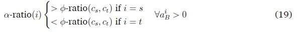
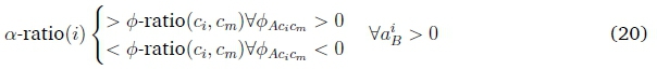
For any two classes c and c_m, the weight gap 4>_AciCm = w_CiA - w_CmAwill either be positive or negative, a value that is consistent for all samples of any specific pair of classes. It can then be shown (see appendix A.1) that if the following holds, all samples i will be classified correctly:

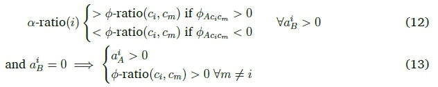
This means that each of the activation ratios must lie in an interval defined by the relevant 0-ratios, in order to achieve perfect classification. Note that the 0-ratios are fixed for all samples, once the network has been trained, and is determined solely by the weight values in the output layer. The role of the nodes up to the last hidden layer can then be viewed as creating activation values that are consistent with the established weight ratios of the final layer. The weight ratios therefore induce an ordering that the activation ratios must reflect. We also expect the activation ratios to fall between a clearly-defined minimum and maximum activation ratio for each class. As there is only a limited number of 0-ratios created, the minimum of one set will form the maximum of another: the range of possible activation values are then in effect partitioned into a set of non-overlapping 'allowed values' per class.

Since activation gaps are created by summing over all active nodes in the previous layer, nodes that are able to separate classes well are re-used, and their ability to separate classes can be analysed by analysing the source of the a-ratios. With this in mind, we also measure the node contribution to the a-ratios of each of the nodes in the layer prior to the summary layer, by first considering only the connecting weights. We define the node-ratio at node n as:

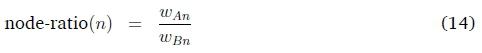
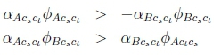
These values will be revisited in Section 5. The conditions for correct classification of a set of samples have some interesting implications. Looking more closely at Equations 9 and 10, these can be rewritten as:

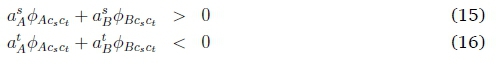
which means that, since the (ReLU-activated) activation values > 0, one of ^_AcsCt or ^_BcsCt will always be negative, and the other positive; or (since ^_BCsCt= -<f>_BctC3) it will always hold that 4>Ac_sct4>BCtC_S> 0, and also that

We already know the a-ratios cannot be negative, which means that it is only the absolute values of Equation 12 that are relevant. Finally, as shown in Appendix A.2, an implication of Equations 15-16 is that it will always hold that:

This does not mean that there is any asymmetry to the roles of A and B here. The inequality of Equation 18 can be rewritten in different ways, as the following are equivalent to Equation 18:

To summarise, in this section we have defined a number of gaps and ratios (Equations 5-8, 14) that are useful for analysing network behaviour; we have described the requirements for perfect classification in terms of weight and activation ratios (Equations 11 -13); and we have looked at some of the other conditions that are also guaranteed to hold for all samples correctly classified (Equations 17-18).

3.3 Network normalisation

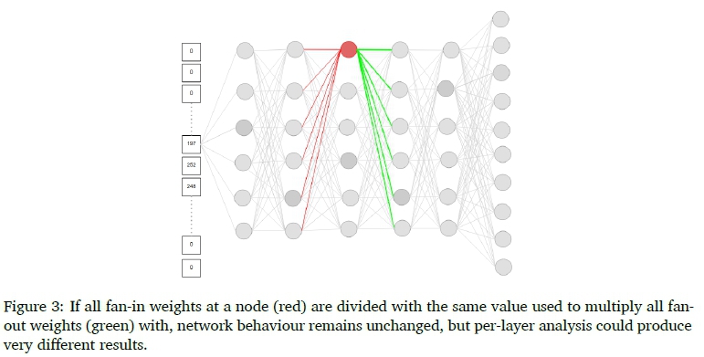
After training and prior to any analysis, the network is weight-normalised to remove potential cross-layer artefacts. Figure 3 demonstrates how it is possible to introduce artefacts that could invalidate a layer-specific analysis, without changing overall network behaviour. If all fan-in weights at a node (red) are divided with the same value used to multiply all fan-out weights (green) with, network behaviour remains unchanged, but per-layer analysis (for example, when comparing weight values in a single layer) could produce very different results.

We therefore perform weight normalisation one layer at a time; normalising the fan-in weight vector per node, and passing this norm along to the fan-out weight vector of the same node at the next layer. Specifically, we calculate the node-specific Euclidean norm of the fan-in weight vector at that node; and use this value to both divide the fan-in weight vector with, and multiply the fan-out weight vector with.

 

4 EMPIRICAL CONFIRMATION

Before demonstrating how the newly-defined values can be useful in analysing network behaviour, we first confirm empirically that the expected relationships hold in practice.

4.1 Trained networks

We train ReLU-activated networks with the architecture of Figure 1 using the MNIST (Lecun et al., 1998) dataset. A fairly standard training setup is used: initialising weights and biases with He initialisation (He et al., 2015); optimising the cross-entropy loss with standard stochastic gradient descent; and performing a grid search of learning rates across different training seeds. No regularisation apart from early stopping is used. Training continues until convergence, and hyper parameters are optimised on a 5,000 sample validation set, using 3 training seeds. We use the same protocol to train networks with hidden layers of 100, 300 and 600 hidden nodes.

Adding a 2-node summary layer does not prevent the networks from achieving fairly good accuracy, as shown in Table 1. The 100-node network does not perform as well, but the networks with 300 and 600 hidden nodes show very similar performance. The 300-node network is selected for analysis, and results are verified to be identical before and after weight normalisation.

At this stage we only report on results where training occurs with the summary layer in place. It is also possible to first train a network, freeze its parameters prior to removing the output layer, and adding a new summary and output layer before training further. Initial results show that this is possible, with the training process particularly fragile, especially if only one hidden layer is used. Additional hidden layers ensure that the combined system trains much more easily, as does adding a third summary node. These results will be explored further in future work: the current analysis focuses solely on an in-place summary layer consisting of only two nodes.

4.2 Confirming analysis equations

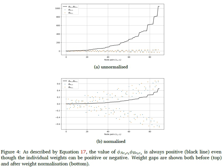
We find that the expected relationships do indeed hold, as illustrated in Figures 4 and 5. Equations were verified for all architectures, but we only show a single architecture here: the 300-node hidden layer model. In Figure 4, all individual weight gaps (Equation 6) as well as the product of the matching weight gaps are plotted for the network before and after normalisation. From Equation 17 this product is expected to always be positive, as observed.

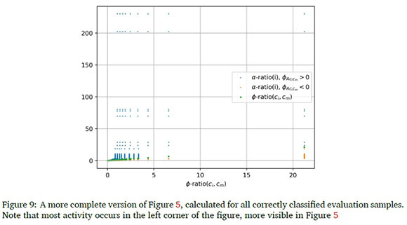
In Figure 5 we extract the activation ratios for 1,000 random correctly classified samples in the evaluation set of the 300-node model, and plot these separately depending on the sign of the relevant weight gap. We also add the samples that were incorrectly classified, and indicate them in red and black, again depending on the weight gap. We confirm that the conditions specified in Equation 12 map directly to correctly and incorrectly classified samples.

 

5 ANALYSIS

In this section, we briefly demonstrate how the gaps and ratios defined in Section 3 can be used to probe the generalisation ability of neural networks. We use the same 300-node model as before when extracting metrics, unless otherwise indicated.

From Equation 12, we expect the activation ratios (Equation 8) to fall between a clearly defined minimum and maximum activation ratio for each class. Since the same weight ratios are re-used across class pairs, the range of possible activation values are in effect partitioned into a set of non-overlapping 'allowed values' per class. This is illustrated in Figure 6. A sample with an activation ratio falling within the allowed values will be correctly classified; outside of this restricted range will cause an error. No ratios are shown for class 6, as it is not classified according to ratios (Equation 12) but according to Equation 13, implying an undefined activation ratio.

Classes that lie on each other's boundaries are more likely to be confusable. In the specific example shown here, the evaluation error was 5.0%. All confusable pairs contributing more than 0.20% absolute of the total evaluation set error (each) are boundary pairs, with the four top confusable pairs being 3-8 (0.48%), 2-8 (0.47%), 4-9 (0.40%) and 7-9 (0.38%).

How are these activation ratios created? We know each active node (in the hidden layer) contributes a value to both the numerator and denominator of the sample-specific activation ratio (a-ratio) in the summary layer, according to (1) its own fan-out weights, and (2) activation value. We are interested in how each hidden node's own node ratio (Equation 14) influences this process. As weighted activation values are added separately to the numerator and denominator of the summary node's a-ratio, it is not immediately obvious what this effect would be. However, by analysing the node ratios and sample sets (Section 2.1) of a well-trained network, we can obtain some intuition in this regard.

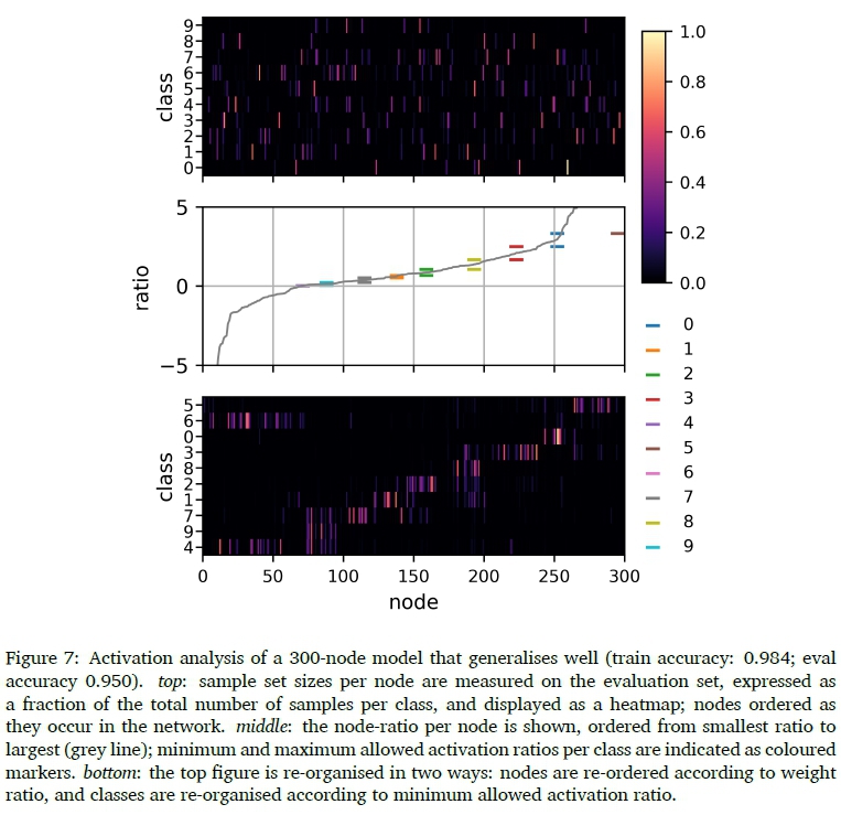
We first calculate the size of the class-specific sample sets at each node, using the same 300-node network as before. This is illustrated in the heatmap at the top of Figure 7, where activation patterns are measured on the full (10,000-sample) evaluation set. Sample set sizes are expressed as a fraction of the total number of samples per class, and nodes are ordered as they occur in the network. It is clear that some nodes activate more strongly for specific classes, but little else is immediately visible. We now measure the node-ratio (difference between weight values linked to a specific hidden node) and plot this from smallest ratio to largest (middle figure, grey line). In the same figure (middle), we indicate the minimum and maximum allowed activation ratios per class. These are the same values as shown in Figure 6. As expected, the node ratios (grey line) and the allowed activation ratios (colour bars) follow exactly the same trend. In the bottom figure, the same values as in the top figure are re-organised in two ways: nodes are re-ordered according to weight ratio, and classes are reorganised according to minimum allowed activation ratio. Now, a much clearer picture starts to emerge: a fairly small number of nodes activate for each class, and these typically have a node ratio that is in the vicinity of the class 'target' ratio, that is, the values between the minimum and maximum allowed activation ratios required for correct classification.

This is by no means the only way in which nodes could have contributed to reaching the target values but, in retrospect, it makes sense that this approach would lead to good generalisation: if the node ratios are fairly similar, any combination of them would have the same average node ratio, and classification would not rely on any specific subset of hidden nodes, but rather a variety of node combinations would all produce the same classification result. In this case, nodes are able to produce the same result either individually, or in collaboration with additional nodes.

We test this intuition on a network that was not well optimised. Specifically we use a seed and learning rate that produce a network that has a similar training accuracy (0.989) but a much poorer evaluation accuracy (0.887). Results look very different, as shown in Figure 8. Sample set constitution is much less organised, and the target weight ratios are clustered closely together. Analysis on either the training or the evaluation set produces comparable results per network. The two networks shown here demonstrate extreme examples of organised vs disorganised behaviour: behaviour on the continuum between these two examples are produced by networks with a variety of generalisation abilities. It is worth noting that training accuracy of both networks are similar, even though it is clear prior to evaluation that one network is expected to generalise better than the other. (Node ratios are determined by weight values, and are not influenced by the data being evaluated.)

 

6 CONCLUSION

We build on results from Davel et al. (2020), which views DNNs as layers of collaborating classifiers, and probe the interplay between the local and global nature of nodes in a hidden layer of an MLP. We ask what the theoretical requirements are for perfect classification of a set of samples from different classes, and answer this question for a simplified architecture, which adds a summary layer prior to the final output layer. In this process, we derive a number of metrics (gaps and ratios) that are useful for probing the inner workings of a neural network.

While the architecture is simplified, it is not trivial: a summary layer can be added to a variety of MLP architectures, which makes the 2-node summary layer less of a restriction than it initially seems. Also, MLPs with multiple hidden layers can be considered as consisting of multiple 3-layer subnetworks stacked on top of one another; it is not immediately clear to what extent the same factors that are important for a 3-layer MLP are important for a subnetwork within a larger structure, but both types of architectures can be probed with the type of analysis described here. The same does not hold for recurrent and residual connections, as these are problematic for theoretical analysis, but convolutional layers can to some extent be analysed as sparse, connected-weight MLPs. The current analysis is restricted to ReLU-activated networks. As the analysis in Davel et al. (2020), which also studied the binary behaviour of individual nodes, was successfully applied to sigmoid-activated networks (with a adjusted definition of what 'on' and 'off' entail) we expect to be able to extend this study to a more diverse set of activation functions as well. This, however, remains future work. All in all, while it should be possible to extend the ideas of this paper to more complex architectures, our first goal is to probe (and eventually characterise) the generalisation ability of straightforward ReLU-activated MLPs.

For a simplified MLP, we have shown how activation ratios are formed prior to the output layer, and how the consistency of these ratios gives rise to the classification ability of a layer. Specifically, we show that nodes act as local 'gap generators' between pairs of samples. These gap generators are formed during gradient descent, when the node-supported cost (Section 2.1) is used to find directions in a layer-specific input space, which are useful for pulling some samples apart and clustering others together. We show that, at the summary level, the ratio of activation values (a single value per sample) aims for a target activation range that is specific to each class. These ratios are formed by nodes in the prior hidden layer, and their manner of use can shed light on the characteristics of networks that we expect to better support generalisation.

Apart from the limited demonstration of the analysis process in Section 5, we have not yet explored the many questions that the current results raise: Which indicators best capture the difference between the good and poor generalisation demonstrated in Figures 7 and 8? To what extent is learning with a summary layer similar to learning without one? From the interaction between sample sets and gaps, some nodes are more general and others more specific: what does this say about the generalisation ability of the network? How are results different if additional layers are added prior to the summary level? In future work we would like to continue to use the analysis proposed here, in order to probe networks for answers to questions such as these.

 

References

Bartlett, P. L., Foster, D. J. & Telgarsky, M. J. (2017). Spectrally-normalized margin bounds for neural networks. Advances in Neural Information Processing Systems, 30, 6240-6249.         [ Links ]

Davel, M. H. (2019). Activation gap generators in neural networks. Proceedings ofthe South African Forum for Artificial Intelligence Research, 64-76.

Davel, M. H., Theunissen, M. W., Pretorius, A. M. & Barnard, E. (2020). DNNs as layers of cooperating classifiers. Proceedings of the Thirty-Fourth AAAI Conference on Artificial Intelligence. https://doi.org/10.1609/aaai.v34i04.5782

Dinh, L., Pascanu, R., Bengio, S. & Bengio, Y. (2017). Sharp minima can generalize for deep nets. Proceedings of the 34th International Conference on Machine Learning (ICML), 10191028.

Goodfellow, I., Bengio, Y. & Courville, A. (2016). Deep learning [http://www.deeplearningbook.org]. MIT Press.

He, K., Zhang, X., Ren, S. & Sun, J. (2015). Delving deep into rectifiers: Surpassing human-level performance on ImageNet classification. Proceedings of the 2015 IEEE International Conference on Computer Vision (ICCV), 1026-1034. https://doi.org/10.1109/ICCV.2015.123

Jiang, Y., Krishnan, D., Mobahi, H. & Bengio, S. (2019). Predicting the generalization gap in deep networks with margin distributions. Proceedings ofthe International Conference on Learning Representations (ICLR).

Kawaguchi, K., Pack Kaelbling, L. & Bengio, Y. (2019). Generalization in deep learning. arXiv preprint, arXiv:1710.05468v5.

Keskar, N. S., Mudigere, D., Nocedal, J., Smelyanskiy, M. & Tang, P. T. P. (2017). On large-batch training for deep learning: Generalization gap and sharp minima. International Conference on Learning Representations (ICLR).

Lecun, Y., Bottou, L., Bengio, Y. & Haffner, P. (1998). Gradient-based learning applied to document recognition. Proceedings ofthe IEEE, 86(11), 2278-2324. https://doi.org/10.1109/5.726791        [ Links ]

Montavon, G., Braun, M. L. & Müller, K.-R. (2011). Kernel analysis of deep networks. Journal ofMachine Learning Research, 12, 2563-2581.         [ Links ]

Nair, V. & Hinton, G. (2010). Rectified linear units improve restricted boltzmann machines. Proceedings ofthe International Conference on Machine Learning (ICML), 807-814.

Neyshabur, B., Bhojanapalli, S., McAllester, D. & Srebro, N. (2017). Exploring generalization in deep learning. Advances in Neural Information Processing Systems, 30.

Raghu, M., Poole, B., Kleinberg, J., Ganguli, S. & Sohl-Dickstein, J. (2017). On the expressive power of deep neural networks. Proceedings ofthe 34th International Conference on Machine Learning (ICML), 70, 2847-2854.         [ Links ]

Shwartz-Ziv, R. & Tishby, N. (2017). Opening the black box of deep neural networks via information. arXivpreprint, arXiv:1703.00810.

Theunissen, M. W., Davel, M. H. & Barnard, E. (2019). Insights regarding overfitting on noise in deep learning. Proceedings of the South African Forum for Artificial Intelligence Research, 49-63.

Vapnik, V. N. (1989). Statistical Learning Theory. Wiley-Interscience.

Zhang, C., Bengio, S., Hardt, M., Recht, B. & Vinyals, O. (2017). Understanding deep learning requires rethinking generalization. Proceedings of the International Conference on Learning Representations (ICLR).

 

 

Received: 18 June 2020
Accepted: 16 November 2020
Available online: 08 December 2020

 

 

1 Note that for a cross-entropy loss function with softmax activations, or for a mean squared error loss function with linear activations, this value reduces to the difference between the target value and the hypothesis value at node c_p. In (Davel et al., 2020) the weight update is expressed in terms of -A for these special cases of loss function (rather than A), resulting in a variant of the same equation.

 

 

A DERIVATION OF ADDITIONAL EQUATIONS

A.1 Requirements for correct classification (Equation 12)

Consider a network with two summary nodes A and B and non-zero weights connecting each summary node to each of the output nodes (one per class), such that all weights from a single summary node are distinct. For any two samples from any two different classes, the weight gap w_CsA - w_ctAwill either be positive or negative. Without loss of generality, assign the samples as s or t such that w_CsA > w_CtA. For these two samples s and t of classes c_sand c_t, let it then hold that

First consider i = s, then:

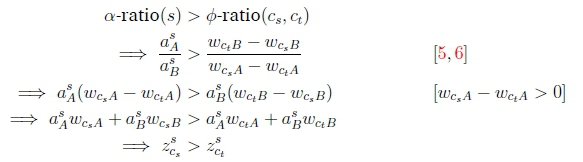
Similarly, if i = t, then

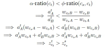
Since 0-ratio(c_s, c_t) = 0-ratio(c_t, c_s), and since a(i) is not influenced by the sign of ^_AcsCt = w_CsA - w_CtA, Equation 19 can be restated as:

This holds for all aⁱ_B > 0. As aⁱ_Bis a non-negative value, the only other option is if aⁱ_B = 0.

If we now assume a positive aⁱ_Aand that all ^_AciCm positive (when i = m), it follows that:

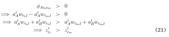
A similar argument shows that if any ^_AciCm is negative and aⁱ_B = 0, no value of aⁱ_Acan result in correct classification.

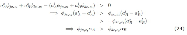
A.2 Equations 17 and 18

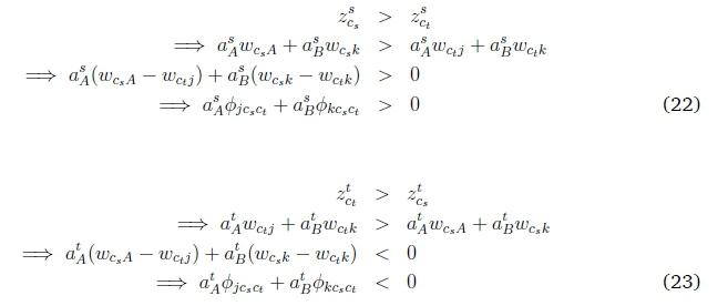
Combining 22 and 23:

 

B SUPPLEMENTARY FIGURES

B.1 Full version of Figure 5

Figure 5 was cropped to show detail. Here we include the full set of results on all correctly classified evaluation samples. Normalised results are shown; pre-normalised and normalised results are similar.

 

 

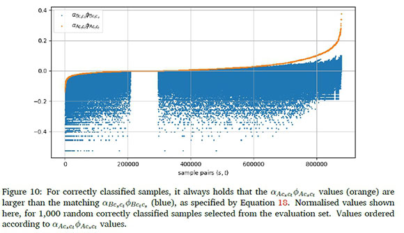
B.2 Demonstration of Equation 18

While Equation 18 is less prominent in this paper than it was in (Davel, 2019), the described relationships still hold for all correctly classified samples, as illustrated in Figure 10.