


Servicios Personalizados
Articulo
 Inglés (pdf)
 Articulo en XML
 Referencias del artículo
Indicadores

Links relacionados
-
 Citado por Google
 -
 Similares en Google
Compartir

 Permalink
South African Computer Journal
versión On-line ISSN 2313-7835
versión impresa ISSN 1015-7999
SACJ vol.32 no.2 Grahamstown dic. 2020
http://dx.doi.org/10.18489/sacj.v32i2.860
RESEARCH ARTICLE
Pairwise networks for feature ranking of a geomagnetic storm model
Jacques P. BeukesI, II; Stefan LotzI, III; Marelie H. DavelI, II
IMultilingual Speech Technologies (MuST), North-West University, South Africa. Email: Jacques P. Beukes jpbeukes27@gmail.com (corresponding), Stefan Lotz slotz@sansa.org.za, Marelie H. Davel marelie.davel@nwu.ac.za
IICentre for Artificial Intelligence Research (CAIR), South Africa
IIISpace Science Directorate, South African National Space Agency (SANSA), Hermanus, South Africa
ABSTRACT
Feedforward neural networks provide the basis for complex regression models that produce accurate predictions in a variety of applications. However, they generally do not explicitly provide any information about the utility of each of the input parameters in terms of their contribution to model accuracy. With this in mind, we develop the pairwise network, an adaptation to the fully connected feedforward network that allows the ranking of input parameters according to their contribution to model output. The application is demonstrated in the context of a space physics problem. Geomagnetic storms are multi-day events characterised by significant perturbations to the magnetic field of the Earth, driven by solar activity. Previous storm forecasting efforts typically use solar wind measurements as input parameters to a regression problem tasked with predicting a perturbation index such as the 1-minute cadence symmetric-H (Sym-H) index. We re-visit the task of predicting Sym-H from solar wind parameters, with two 'twists': (i) Geomagnetic storm phase information is incorporated as model inputs and shown to increase prediction performance. (ii) We describe the pairwise network structure and training process - first validating ranking ability on synthetic data, before using the network to analyse the Sym-H problem.
CATEGORIES: • Computing methodologies ~ Neural networks • Applied computing ~ Earth and atmospheric sciences
Keywords: space weather, input parameter selection, neural networks
1 INTRODUCTION
In this work we present an adaptation to the fully-connected feedforward neural network (FFNN) structure to allow for the ranking of a set of inputs during training, with no significant trade-off in performance. We apply this network to a space weather regression problem and show that the ranking it produces corresponds to the underlying physical processes involved.
This work builds on Lotz et al. (2019), where the "pairwise" network architecture was first introduced. We improve the architecture and ranking procedure by adding summary nodes to the pairwise network and taking activation values into account when ranking, instead of only the weights. We also propose parameter pruning as a way to improve the model's ranking capability. As an extended version of Lotz et al. (2019), relevant content is repeated here.
Section 2 provides a short overview of space weather in the context of this paper and a description of the input and target parameters considered for this study. Previous work on the interpretability of artificial neural networks that relates to this study is also mentioned. In Section 3, we describe the process followed to construct the data sets, and Section 4 stipulates the architecture and training procedure of the models considered in this work. In Section 5, we validate the pairwise procedure on two artificial problems with different levels of complexity before revisiting the space weather problem in Section 6. Section 7 discusses the limitations of and possible future improvements to our approach, followed by the conclusion in Section 8.
2 BACKGROUND
Violent eruptions of electromagnetic energy (solar flares) and charged plasma (coronal mass ejections or CMEs) on the solar surface are propagated through interplanetary space and can impact the Earth's geomagnetic field. These perturbations can result in the disruption of various kinds of technological systems such as satellite (Béniguel & Hamel, 2011) and HF radio communications (Frissell et al., 2019) and power grids, oil pipelines and other ground-based conductor networks (Boteler, 2001; Trichtchenko & Boteler, 2002). These effects are collectively known as "space weather". Due to the adverse effects on critical technological systems, major efforts are underway to monitor and predict space weather accurately (Oughton et al., 2019).
Multi-day intervals of disruption to the geomagnetic field are known as geomagnetic storms (Gonzalez et al., 1994) and their severity is quantified by indices that measure the net disturbance to the geomagnetic field. The direct cause of geomagnetic storms is the injection of energetic solar wind particles into the magnetosphere (the region of space around Earth dominated by the geomagnetic field) and the increased degree of coupling between the solar wind and magnetospheric plasmas. The prediction of a geomagnetic disturbance (GMD) index from solar wind data lends itself to modelling as a regression problem, and many attempts to do this have been made (Gruet et al., 2018; Lotz et al., 2015; Siscoe et al., 2005; Wintoft et al., 2005). One such GMD index is the symmetric-H (Sym-H) index, which is constructed from measurements at multiple magnetic observatories on Earth. (See Section 2.3 for more detail on the Sym-H index). Our aim is to predict the Sym-H index (on Earth) from solar wind parameters (as measured in space).
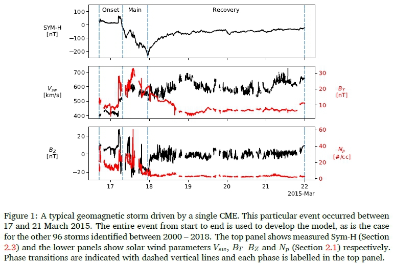
Figure 1 shows the progression of a geomagnetic storm over about four days. The top panel shows the Sym-H index and the lower two panels show solar wind parameters measured by the Advanced Composition Explorer (ACE) spacecraft. All values are shifted in time to the estimated position of the magnetospheric bow shock nose (BSN) position. This storm was due to a single CME impacting the magnetosphere and the passage of ejecta past the spacecraft is recognisable as the increases in speed, density, and fluctuations of the interplanetary magnetic field (IMF). A typical geomagnetic storm is seen in the Sym-H curve, with the onset phase indicating the arrival of the CME on 17 March, moving into the main phase as the IMF turns southward (Bz < 0), resulting in increased coupling between the solar wind and magneto-sphere. After the IMF turns northward (Bz > 0) and the bulk of the disturbed solar wind plasma has passed, the magnetosphere can recover.
Within this context, we revisit the regression problem - where we task a feedforward neural network to predict Sym-H from solar wind parameters - with two important changes: Firstly, an adapted network topology is designed to enable the analysis of input parameter weights. The aim is to use the weight adaptations performed by the model training procedure to rank input parameters according to importance. Secondly, we show that the inclusion of storm phase as an input parameter to the model increases prediction performance. We know that different physical phenomena are at play during different phases of a geomagnetic storm. Finally, we show how the input parameter rankings change when restricting the model to only one storm phase, further demonstrating the utility of analysing parameter importance to gain insight into the problem at hand, beyond merely seeking accurate predictions.
Prior to addressing the task as just described, we demonstrate the development of pair-wise networks and the selection of input parameters on two synthetic regression problems: a straightforward function of a small set of parameters (Section 5.1) and regression problems from space weather (Section 5.2). The latter task models a synthetic parameter, Akasofu's e, which is derived from solar wind parameters. The rest of this section is dedicated to describing the space weather-related inputs and outputs.
2.1 Solar Wind Parameters
Several plasma and magnetic field parameters are included in this study, all contributing to some extent to the dynamics involved in driving a geomagnetic storm:
VswSolar wind speed [km/s] is the bulk speed of the plasma moving across the spacecraft.
NpProton number density [#/cc] measured in particles per cubic centimetre indicates the particle density of the plasma. Coronal mass ejecta are usually denser than the ambient solar wind plasma.
PdDynamic flow pressure [nPa] is the flow pressure of the solar wind and is linearly related to NpVs2W.
EMMerging electric field in the solar wind [mV/m] serves as an indication of the coupling between the solar wind and magnetospheric plasmas and is linearly related to -VswBZ.
Bx,y,z, BTThe three components of the IMF, measured in nT, and the total field BT.
2.2 Akasofu's e
This parameter serves as an indication of the amount of energy (in Watts) deposited by the solar wind into the magnetosphere (Koskinen & Tanskanen, 2002). It is defined by
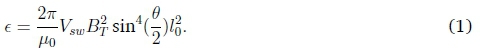
with 0 = tan (BY/BZ) the clock angle of the IMF, μ0 the vacuum permittivity, and l0a scaling factor determined empirically. In Section 5.2 a simplified version of this parameter is modelled, with solar wind parameters as input:
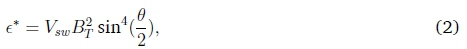
The e* parameter simply avoids the scaling constants, but the relationship with solar wind parameters remains intact. This regression problem enables the evaluation of our pairwise network on a complex but known relationship between input and output parameters, utilising real-world data.
2.3 Symh-H index
The target or output parameter to the regression problem described in Section 6 is the symmetric H (Sym-H) index. This is an index calculated at 1-minute cadence, derived from the horizontal (with regard to the Earth's surface) component of the geomagnetic field measured at 11 middle latitude magnetic observatories. The calculation is based on averaging disturbances to the H-index at longitudinal pairs of stations. Sym-H serves as an indication of the strength of the ring current (Moldwin, 2008) which circles the Earth and is the main driver of magnetic storm activity at middle latitudes.
The physical phenomena relating Sym-H to solar wind plasma are reasonably well understood by space physicists, but an exact, quantitative transfer function relating solar wind parameters to Sym-H is not known.
2.4 Related work
Several attempts have been made to extract feature ranking from deep neural networks. A prominent direction is attribution methods, such as Integrated Gradients (Sundararajan et al., 2017), DeepLIFT (Shrikumar et al., 2017) and Layer-wise Relevance Propagation (LRP) (Bach et al., 2015), that assign an importance score to each input feature of a network. Attribution methods do not form part of the model's structure and can be readily applied to a wide range of architectures, however this also means that these methods only approximate model behaviour.
In contrast, the pairwise network introduced in this work are intrinsically interpretable, that is, the structure of this network allows for feature ranking. Similar architectures exist in the literature, most of which are based on generalised additive models (GAMs) (Hastie & Tibshirani, 1986), first introduced as "progression pursuit regression" (Friedman & Stuetzle, 1981). GAMs take the form:
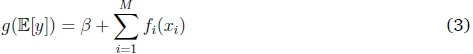
where y is the target, x = (x1,x2,... ,xM) is the input with M features, g is the link function and fiis a univariate shape function.
Generalised Additive Neural Networks (GANNs) were introduced in (Potts, 1999) and was the first attempt to use neural networks for approximating the shape functions of GAMs. However, the GANNs used in (Potts, 1999) were not trained with back-propagation and only consisted of a single hidden layer. Neural Additive Models (NAMs) (Agarwal et al., 2020) improve GANNs significantly with several architectural and optimisation changes. GAMI-Net (GAMs with structured Interactions) (Yang et al., 2020b) essentially adds pairwise interactions to GANNs, approximating:

Neural Interaction Transparency (NIT) (Tsang et al., 2018) is a framework that produces the same model as GAMI-Net, but by disentangling interactions within a FFNN. The Explainable Neural Network (xNN) (Vaughan et al., 2018), Adaptive xNN (AxNN) (Chen et al., 2020) and Enhanced xNN (ExNN) (Yang et al., 2020a) are all based on the Generalised Additive Index Model (GAIM):

where wiare known as the projection indices.
Except for GANN (1999), NIT (2018) and xNN (2018), all of these techniques were developed in parallel with ours, with ExNN, GAMI-Net, AxNN and NAM (preprint) published in 2020.
3 DATA SET
The space weather data set comes from a public source (Section 3.1) with specific events of interest selected for model building, as described in Section 3.2.
3.1 Source
Data is collected from the High Resolution OMNI (HRO) data set1, which combines measurements taken from several satellites and includes both solar wind parameters and several geomagnetic disturbance indices, of which Sym-H is one.
This data set is already preprocessed in the following steps: Solar wind measurements taken at 16 or 64-second cadence (depending on the instrument) are averaged to 1-minute values and shifted in time to the estimated position of the magnetospheric bow shock nose (BSN). This ensures that the propagation time from the first Lagrange point (L1) to the BSN does not have to be incorporated into model development.
3.2 Event selection
The data set consists ofsolar wind and Sym-H data, at 1-minute cadence, from the period 2000 - 2018. This period includes almost two full solar activity cycles, but since geomagnetic storms are fairly rare events, using all available data would result in a very unbalanced data set, with the storm periods being under-represented. Therefore, only intense geomagnetic storms, those with minimum Sym-H < - 100 nT, were selected out of the 19 year period.
The event selection algorithm is described in Lotz and Danskin (2017). Using this method 97 storms are identified between 2000 and 2018, resulting in 396,164 minutes of data (excluding missing values) out of the ~ 9.9 x 10⁶ minutes spanning the 19 year interval. In this set, the average storm has a duration of 5,000 minutes (~ 3.5 days) with a standard deviation of 2,200 minutes (~ 1.5 days). The selection algorithm was developed for practical use and built to consider closely separated events as a single event, in order to focus on the effect of the event rather than the cause.
The collection of distinct storms are used to divide the data into training (67 storms), testing (15 storms) and validation (15 storms) sets. Keeping storm intervals separate ensures that the three sets are truly independent - every storm interval is wholly contained in only one of the three data sets. The training set is used during training to adapt weights through gradient descent, the validation set is used to determine the model's performance after each epoch, and the test set serves as the independent out-of-sample data set on which the model's performance is ultimately calculated. The entire data set is standardised by subtracting the mean and scaling to unit variance, where both scalers are calculated on the training set.
Within each storm, the onset, main and recovery phases are identified by searching for (i) the interval around the positive increase in Sym-H (onset phase), (ii) the rapid decrease to storm minimum (main phase), and finally (iii) the recovery period from the minimum Sym-H until the end of the event. These identifiers are important because there are different physical processes involved in the various storm phases.
4 MODEL DEVELOPMENT
Two different types of architectures are utilised, a standard fully-connected FFNN and a "pair-wise" neural network, detailed below (Section 4.1). The same process is utilised to optimise all networks, as described in Section 4.4.
4.1 The pairwise network
A fully-connected feedforward network layout mixes signals from all inputs as information flows through the hidden layers to the output. This enables the training procedure to utilise all the different combinations of input parameters to find an efficient solution. Analysis of these sets of combinations is prohibitively complex since, from the first layer of hidden nodes, every node is directly or indirectly connected to every input parameter. Selectively removing some connections from the input layer to the first hidden layer results in distinct combinations of inputs to be fed to the subsequent hidden layers of a network.
The pairwise network, as originally introduced in (Lotz et al., 2019), is constructed according to the following procedure. Given a model with M input parameters, H hidden nodes in a single hidden layer, and a single output node:
1. Find all possible distinct pairs of inputs {Xi, Xj} (i = j) in the list {X1,X2,..., XN}. Say there are P such pairs, and note that {Xi,Xj} = {Xj,Xi}.
2. Divide the set of hidden nodes into P distinct groups.
3. For each group, create a sub-network by fully connecting each pair of inputs to its corresponding group of hidden nodes.
4. For each sub-network fully connect the nodes of the final hidden layer to a single node (the summary node).
5. Fully connect the summary nodes of each sub-network to a single output node.
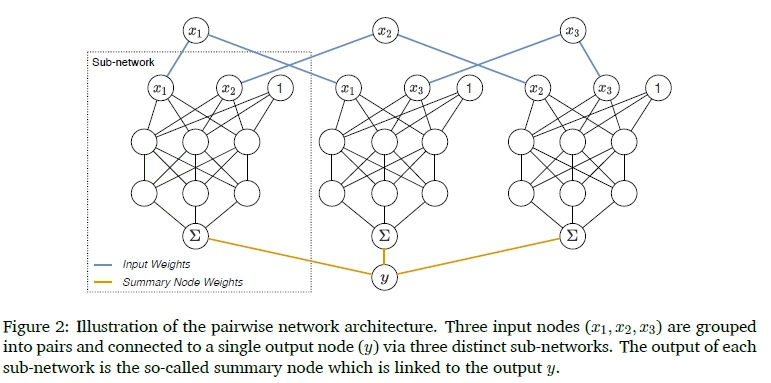
Figure 2 shows the layout of this network. The input weights in the first layer of the pairwise network is set to have a value of 1 and frozen so as not to update during training. Biases are added to the second layer of the pairwise network and ReLU activation functions are placed after every layer except the first (input), second-last (summary) and final layer. All sub-networks are initialised to have identical weight values between sub-networks. This is achieved by randomly initialising a single sub-network and then duplicating its weights to all other sub-networks. This network is identical to the one described in (Lotz et al., 2019), apart from the more careful weight initialisation performed here.
4.2 Ranking procedure
The input parameter ranking process improves on the one described in (Lotz et al., 2019). It is performed after training by passing a set of samples through the network and then capturing the activation values of each sub-network's summary node. For any given sample, the output node value is the weighted sum of the summary node activation values. The reasoning is that the magnitude of the weighted summary node activation values gives an indication of sub-network importance for that sample. When averaging over all samples, the importance of each sub-network can be estimated for the particular set. We refer to this as the weighted summary node activation distribution.
It can happen that the training algorithm completely prunes one of the inputs from a subnetwork. We renamed such sub-networks to have the same name as the remaining input.
4.3 Pruning procedure
In addition to the standard pairwise network, we also investigate iterative pruning of the model's weight parameters, similar to the method described in (Han et al., 2015). This increases the model's ranking capability by forcing the network to be more sparse.
The procedure we implemented is as follows: we first train the network to completion, and then prune p% of the smallest unpruned weights according to their magnitude, by setting their values to 0 and freezing them so that they do not get updated in subsequent training steps. The remaining weights are then retrained to completion. Pruning and training are repeated until the network reaches the desired level of sparsity or until the network's performance on the validation set falls below a predetermined threshold from the best value of the preceding iterations. This threshold value sets the trade-off between sparsity and performance.
4.4 Model development
Two distinct network layouts are investigated in this work: standard feedforward networks and the pairwise network layout described above. The baseline model (hereafter labelled B1) is a fully connected FFNN with solar wind parameters as input and Sym-H as output. Model B1 is trained with the 8 solar wind inputs, two hidden layers of 10 nodes each and a single output node (Sym-H).
To enable the model to capture time information, we add temporally shifted versions of each parameter to the set of inputs. The magnetospheric response to solar wind energy input is non-linear in time and there are non-zero decay times determining the response of the ring current (and Sym-H index) (Moldwin, 2008; Vassiliadis et al., 1999). Therefore we include a time-shifted version of input parameters. For each input parameter Xt, measured at time t, another input Xt-mis added, doubling the number of inputs of model B2 to 16. In this case, we let m = 270 minutes, chosen by a parametric search of shifts. Applying this time shift resulted in a marked increase in performance (see Section 6). Note that a constant shift size is a limitation of the model because it incorrectly assumes that the time scale of energy deposition and magnetospheric processes is identical for all geomagnetic storms.
A further improvement is made by adding categorical input parameters to indicate phase since different physical processes are at play during the three storm phases. The relevant phase indicator is set to 1 when the appropriate phase (onset, main or recovery) is in progress, and set to 0 at other times. Therefore, model B3 has 8 + 3 = 11 input parameters.
All Pi models are the pairwise equivalents of the Bi models. Both the Bi and Pi models are trained with Adam (Kingma & Ba, 2015) as the optimiser and mean squared error (MSE) as the loss function. Correlation between the predicted and observed output is used as a performance metric. All optimisation decisions are based on the model's performance on the validation set. Early stopping is implemented by selecting models with the largest validation correlation. Correlation and MSE are correlated for this task, so either one could be used as a performance metric (Beukes, n.d.). An analysis using MSE is available in (Beukes, n.d.).
Extensive probing showed that weight decay, batch normalisation and learning rate schedulers make little to no improvement to the performance, therefore none of these are used. It was also found that smaller mini-batches have better performance, so a mini-batch size of 64 is chosen. Increasing the network width or depth does not improve performance, therefore the mentioned network sizes are chosen as such in favour of computational efficiency. A grid search is done to determine the best learning rate. Three initialisation seeds are considered for both the Bi and the Pi models. The test results of these models are discussed in Section 6.
5 VALIDATION ON SYNTHETIC DATA
To validate the pairwise network's ranking capability, we investigate two synthetic problems, with different degrees of complexity. We use the model development process described in Section 4.4 and train pairwise networks with 2 hidden layers and 10 hidden nodes per subnetwork.
5.1 Synthetic example 1: y = f (x)
Here we generate 3 data sets with input features sampled from a standard normal distribution

and target values
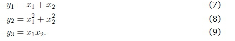
After generating target values, the data set is standardised by removing the mean and scaling to unit variance. Each data set consists of 400 training and 100 validation samples.
We experimented with several pruning amounts p = (10,15,20,25,30} and found that pruning more parameters per iteration tends to hurt ranking capability. On the other hand, small values require more pruning iterations to reach the desired level of sparsity. Here, we report on p = 20.
For each data set, a pairwise network is trained over 4 initialisation seeds and in every case, the network reached above 0.92 correlation on the validation set. Figures 3(a), 3(b) and 3(c) show the weighted summary node activation distributions when passing the respective training sets through trained pairwise networks.
5.2 Synthetic example 2: Akasofu's t
Here we generate target values from a subsection of the Sym-H data set, as described in Sections 2.2 and 3, using the simplified t* parameter (Equation 2). We test two sets of input parameters: {Vsw,BT,0,r} and {Vsw,BT,BY,BZ,r}, where r ~ N(0,1). In both cases, the network is expected to identify the random variable r as an unwanted parameter since it does not form part of the data generation. (Refer to Section 2.1 for a description of the solar wind parameters used here.)
Optimisation produces pairwise networks with a validation correlation above 0.9. Figures 3(d) and 3(e) shows the weighted summary node activation distributions of pairwise networks trained with the respective sets of input parameters.
5.3 Discussion of synthetic examples
For almost all seeds of each synthetic example (see seed 1 in Figure 3(d) for the exception), the predominant part of the weighted summary node activation distribution is occupied by pairs that do not contain the unwanted variable. It is therefore clear that the pairwise network is able to identify the parameters that influence the target value, and can suppress noise very effectively.
Notice the contrast between the y = xxx2problem (Figure 3(c)) and the other two problems of synthetic example 1 (Figures 3(a) and 3(b)). For this problem, both xxand x2are required as inputs for a sub-network to be ranked the highest, but for the other two cases the network is able to produce the output from sub-networks where only one of the required inputs are present. This is to be expected, as the final layer of the pairwise network can easily model addition, but not multiplication.
6 RESULTS
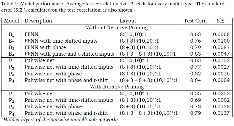
The performance of the baseline (Bi) and pairwise (Pi) models are listed in Table 1. We first consider the ability of the models to solve the task itself (Sections 6.1 and 6.2), before considering their parameter ranking ability (Section 6.3) and what this means. Pairwise results are shown for training both with and without iterative pruning.
6.1 Baseline model
Without phase or time-shifted inputs, the optimal baseline model (B1) has a 0.63 test correlation. By adding time-shifted inputs (B3) or phase (B2), the performance increases to 0.76 and 0.79, respectively. With both phase and time-shifted inputs added (B4), the model reaches a test correlation of 0.83.
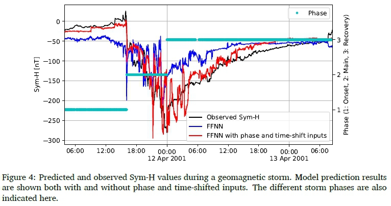
Figure 4 shows an example of Sym-H predicted by models B1 and B4 during a geomagnetic storm. It clearly shows the advantage of adding time-shifted parameters and phase information to the set of inputs, especially during the onset and recovery phases.
6.2 Pairwise network
With no phase or temporal information (P1), the pairwise model has a 0.63 correlation on the test set. By adding time-shifted (P2) or phase (P3) inputs, the test correlation increases to 0.77 and 0.82, respectively. With both phase and time-shifted (P4) inputs, the test correlation reaches 0.84.
When pruning iteratively, the resulting pairwise network has between 70% and 90% fewer parameters, but at the cost of performance. In all cases, the iteratively pruned pairwise network has lower test correlation than the baseline model.
6.3 Input parameter ranking through pairwise network
The pairwise network P1 is developed with (i) the entire data set, and (ii) with the dataset divided according to the 3 storm phases. This enables the ranking of input pairs in general and for separate storm phases. This is to see if the input ranking via the pairwise networks reflects the known differences in physical phenomena at play during the different storm phases. In both cases the best performing pairwise model is used.
Similar to Section 5, we pass the training set through the network to extract weighted summary node activation distributions, but with all 8 input parameters in pairs of2, the graphs become overly complex. As an alternative, we use this distribution to estimate attribution values for each input parameter and present the results in Tables 2, 3, 4 and 5.
Input parameter attribution values are determined by dividing each sub-network's portion of the weighted summary node activation distribution equally between every unpruned input connected to the sub-network (thereby assuming they contribute equally) and then summing over all sub-networks. It was found that pairwise networks rank poorly when trained without iterative pruning. In the following sections, we only show ranking results for pairwise networks trained with iterative pruning.
6.4 Interpretation of the input parameter selection
In this section, we evaluate the ranking input parameters performed by the pairwise network models against our current understanding of the physical processes involved in the solar wind-geomagnetic field coupling during geomagnetic storms. The ranking capability of the model when trained on the bulk data set is discussed and in the subsequent subsections, model performance is discussed for each of the three phases of geomagnetic storms.
Table 2 shows the input parameter ranking according to the attribution method described in section 6.3. The rankings vary by seed, but as explained below, the top-ranked parameters for each seed points to similar physical processes at work. In each of the three sets of ranks the top seven parameters (out of 16) are related to the dynamic pressure applied by the solar wind to the magnetosphere, i.e. Vsw, Npand BT, or the coupling of the solar wind plasma to the magnetospheric plasma (EM, Bz, and Vsw). It is peculiar that the dynamic pressure parameter Pd (~ NpVs2W) does not feature in the top-ranked input parameters. This may be due to the influence of Vswand Npbeing strong indicators of solar activity and the training algorithm not responding to features duplicated by Pd, or that the relationship between Sym-H and Vswis linear rather than quadratic. The X and Y components of the IMF (Bxand BY) consistently achieve low rankings. This is to be expected as these parameters indicate the sun-ward (X) and ecliptic (Y) components of the IMF. Only the Z-component is directly related to reconnection between the IMF and geomagnetic field.
In most cases, both the instantaneous (X[t]) and the time-shifted (X[t - 270]) versions of parameters achieve high ranking scores. This confirms that the current Sym-H values are driven by current and previous conditions in the solar wind. This is indeed the case since the solar wind-magnetosphere coupling depends on various processes, with different time dependencies.
To summarise, the model correctly separates the important parameters from those less important to the regression problem in the context of a set of highly mutually correlating input parameters. All the solar wind parameters are characteristics of the same volume of plasma and its associated magnetic field. Furthermore, duplicated information due to parameters representing similar physical parameters is not reflected in the ranking.
6.4.1 Onset phase results
On average it is Vswand Npthat dominate the onset phase, with BZin third place. It makes sense that pressure-related terms (i.e. Npand Vsw) would dominate, since for intense storms the onset phase is usually characterised by the so-called storm sudden commencement - caused by a sudden increase in solar wind dynamic pressure which compresses the dayside magnetosphere, resulting in an increase in horizontal magnetic field measured on the ground (Gonzalez et al., 1994). This increase manifests in Sym-H as a significant upward pulse lasting minutes to hours. The onset phase is defined as the period before significant reconnection takes place and hence the BZand EMcomponents do not play a big role here, although the sudden increase in pressure is usually accompanied by an increase in total IMF and Z-component of IMF (see Figure 1 just before the start of the main phase period).
6.4.2 Main phase results
Storm main phase is defined by the magnetic reconnection between the IMF and geomagnetic fields which happens when BZturns negative, allowing field lines at the day side mag-netopause to merge with IMF lines. Therefore the high rankings of BZand EMin Table 4 is expected (Vassiliadis et al., 1999). During this time the solar wind speed Vswacts as a modulator of the energy input into the open magnetosphere. It is interesting that, on average, it is EMand both its constituent parameters BZand Vswthat are highly ranked. On the other hand, during the onset phase the pressure-related terms Npand Vswwere both ranked high but not the combined parameter Pd. Again, this points to Sym-H being linearly correlated to Vsw, rather than a higher order relationship.
6.4.3 Recovery phase results
During storm recovery, it is the absence of energy input from the solar wind that allows the magnetosphere to recover by various internal wave-particle interactions that drain energy from particle populations (McPherron, 1995; Vassiliadis et al., 1999). After a CME passes, the solar wind speed gradually decreases to ambient level and the fluctuations in the IMF decrease significantly. Here the top-ranking inputs are BT, Pd, and BZ. Pdachieves a very high score for Seed 3, but zero scores for Seed 1 and 2, resulting in the high average score. Note further that for Seed 1 both Npand Vswachieve relatively high scores, with Pdrated zero. Thus for this phase, there seems to be an equivalence between Pdand (Vsw, Np), suggesting that perhaps the Sym-H-Vsw relationship is of higher order than for onset and main phases. Total IMF BT serves as a general indicator of disturbed solar wind and is usually characterised by a gradual decrease during the recovery phase. During CME-driven solar wind disturbances it is typically the Z-component that varies more coherently than the BXor BYcomponents, and therefore there is high correlation between BZ and BT, especially during the main and recovery phases.
7 DISCUSSION
This investigation confirms that neural networks are a viable option for predicting a geomagnetic storm index (i.e. Sym-H) from solar wind parameters alone. The simplest model is able to reach an average test correlation of 0.63. By adding phase and temporal information, the average performance increases to 0.83. The proposed pairwise network achieved approximately the same predictive performance (0.84) as the standard feedforward neural network when trained without pruning.
Iteratively pruning the network during training, adds the benefit of ranking the importance of input parameters at the cost of a decrease in performance and an increase in training time. The pruning process is computationally expensive since the network has to be retrained at every pruning iteration. Another shortcoming of the current pairwise network is that its use is limited to smaller tasks: since every combination of input pairs receives a sub-network, the model grows quickly, becoming unwieldy.
There are several improvements to be made. First of all, to reduce the training time, the pruning algorithm can be adapted to stop at an earlier stage where the drop in performance is less severe, but the level of sparsity ensures good ranking. Optimal pruning strategies have not yet been investigated. In addition, alternative methods for enforcing sparsely-trained networks can be considered. For example, one can add a term to the loss function that ensures sparsity in certain layers of the network. This approach will decrease training time since no pruning iterations are required. Another improvement would be to add existing attribution methods to the ranking procedure. For example, DeepLIFT (Shrikumar et al., 2017) or Integrated Gradients (Sundararajan et al., 2017) can be used to get an estimate for the importance of each input parameter to a sub-network.
In this work we base the pairwise network on the FFNN for its relative simplicity with regards to both implementation and analysis. Architectures that are more suitable for sequence modelling, such as recurrent or convolutional neural networks, can be incorporated in future versions of the pairwise network.
8 CONCLUSION
In this work we illustrated how domain knowledge can increase the performance of a neural network-based model on a well-known regression problem, and that careful model design can inform domain knowledge. This is of particular relevance in the current age of rapidly increasing machine learning capability, where researchers and domain experts are becoming increasingly cognisant of the dangers of well-performing but unexplainable models. Our contribution in this regard is to introduce a novel neural network that implements a form of intrinsic interpretability through layout constraints to allow an, admittedly crude, way of feature ranking.
Revisiting the well-known solar wind-Sym-H regression problem, we showed that adding storm phase and time-shifted solar wind parameters increases model performance, as would be expected given the current understanding of the problem. For our pairwise network, it was shown that (i) the architectural modifications do not decrease performance when compared to a simple FFNN, but that (ii) the training procedure followed to produce networks with good ranking ability might decrease the performance. Lastly, it was shown that (iii) the rankings, calculated by taking the weighted summary node activation values, generally agree with the current understanding of the problem.
Further development of the pairwise network introduced here will concentrate on a more rigorous analysis of the ranking procedure and an improvement in the architecture and training algorithm to produce networks with better performance and ranking capability. A more rigorous analysis on a broader range of synthetic data sets are required, but eventually, the development will shift to the application of these ideas to other, less well-understood tasks.
References
Agarwal, R., Frosst, N., Zhang, X., Caruana, R. & Hinton, G. E. (2020). Neural additive models: Interpretable machine learning with neural nets. arXivpreprint, arXiv:2004.13912. http://arxiv.org/abs/2004.13912
Bach, S., Binder, A., Montavon, G., Klauschen, F., Müller, K. R. & Samek, W. (2015). On pixel-wise explanations for non-linear classifier decisions by layer-wise relevance propagation. PLoS ONE, 10(7). https://doi.org/10.1371/journal.pone.0130140 [ Links ]
Béniguel, Y. & Hamel, P. (2011). A global ionosphere scintillation propagation model for equatorial regions. Journal of Space Weather and Space Climate (JSWSC), 1(1), A04. https://doi.org/10.1051/swsc/2011004 [ Links ]
Beukes, J. P. (n.d.). Interpretability of deep neural networks for SYM-H prediction (Master's thesis) [Inpreparation]. North-West University. South-Africa, Potchefstroom.
Boteler, D. H. (2001). Assessment of geomagnetic hazard to power systems in Canada. Natural Hazards, 23(2), 101-120. https://doi.org/10.1023/A:1011194414259 [ Links ]
Chen, J., Vaughan, J., Nair, V. & Sudjianto, A. (2020). Adaptive explainable neural networks (Axnns). SSRNElectronic Journal. https://doi.org/10.2139/ssrn.3569318
Friedman, J. H. & Stuetzle, W. (1981). Projection pursuit regression. Journal of the American Statistical Association, 76(376), 817-823. https://doi.org/10.1080/01621459.1981.10477729 [ Links ]
Frissell, N. A., Vega, J. S., Markowitz, E., Gerrard, A. J., Engelke, W. D., Erickson, P. J., Miller, E. S., Luetzelschwab, R. C. & Bortnik, J. (2019). High-frequency communications response to solar activity in September 2017 as observed by amateur radio networks. Space Weather, 17(1), 118-132. https://doi.org/10.1029/2018SW002008 [ Links ]
Gonzalez, W. D., Joselyn, J. A., Kamide, Y., Kroehl, H. W., Rostoker, G., Tsurutani, B. T. & Vasyliunas, V. M. (1994). What is a geomagnetic storm? Journal of Geophysical Research, 99(A4), 5771. https://doi.org/10.1029/93ja02867 [ Links ]
Gruet, M. A., Chandorkar, M., Sicard, A. & Camporeale, E. (2018). Multiple-hour-ahead forecast of the Dst index using a combination of long short-term memory neural network and Gaussian process. Space Weather, 16(11), 1882-1896. https://doi.org/10.1029/2018SW001898 [ Links ]
Han, S., Pool, J., Tran, J. & Dally, W. J. (2015). Learning both weights and connections for efficient neural networks. arXiv:1506.02626. https://arxiv.org/abs/1506.02626
Hastie, T. & Tibshirani, R. (1986). Generalized additive models. Statistical Science, 1(3), 297310. https://doi.org/10.1214/ss/1177013604 [ Links ]
Kingma, D. P. & Ba, J. L. (2015). Adam: A method for stochastic optimization. International Conference on Learning Representations (ICLR), arXiv:1412.6980v9. https://arxiv.org/abs/1412.6980v9
Koskinen, H. E. & Tanskanen, E. I. (2002). Magnetospheric energy budget and the epsilon parameter. Journal of Geophysical Research: Space Physics, 107(A11). https://doi.org/10.1029/2002JA009283 [ Links ]
Lotz, S. & Danskin, D. W. (2017). Extreme value analysis of induced geoelectric field in South Africa. Space Weather, 15(10), 1347-1356. https://doi.org/10.1002/2017SW001662 [ Links ]
Lotz, S., Heilig, B. & Sutcliffe, P. (2015). A solar-wind-driven empirical model of Pc3 wave activity at a mid-latitude location. Annales Geophysicae, 33(2), 225-234. https://doi.org/10.5194/angeo-33-225-2015 [ Links ]
Lotz, S., Beukes, J. P. & Davel, M. H. (2019). Input parameter ranking for neural networks in a space weather regression problem. Proceedings of the South African Forum for Artificial Intelligence Research (FAIR), 133-144. http://ceur-ws.org/Vol-2540/FAIR2019_paper_50.pdf
McPherron, R. L. (1995). Introduction to Space Physics. Cambridge University Press.
Moldwin, M. (2008). An introduction to space weather. Cambridge University Press. https://doi.org/10.1017/CBO9780511801365
Oughton, E. J., Hapgood, M., Richardson, G. S., Beggan, C. D., Thomson, A. W., Gibbs, M., Burnett, C., Gaunt, C. T., Trichas, M., Dada, R. & Horne, R. B. (2019). A risk assessment framework for the socioeconomic impacts of electricity transmission infrastructure failure due to space weather: An application to the United Kingdom. Risk Analysis, 39(5), 1022-1043. https://doi.org/10.1111/risa.13229 [ Links ]
Potts, W. J. E. (1999). Generalized additive neural networks. Proceedings of the Fifth ACM SIGKDD International Conference on Knowledge Discovery and Data Mining (KDD '99), 194-200. https://doi.org/10.1145/312129.312228
Shrikumar, A., Greenside, P. & Kundaje, A. (2017). Learning important features through propagating activation differences. arXiv:1704.02685. https://arxiv.org/abs/1704.02685
Siscoe, G., McPherron, R. L., Liemohn, M. W., Ridley, A. J. & Lu, G. (2005). Reconciling prediction algorithms for Dst. Journal ofGeophysical Research: Space Physics, 110(A2), A02215. https://doi.org/10.1029/2004JA010465 [ Links ]
Sundararajan, M., Taly, A. & Yan, Q. (2017). Axiomatic attribution for deep networks. International Conference on Machine Learning (ICML), arXiv:1703.01365. http://arxiv.org/abs/1703.01365
Trichtchenko, L. & Boteler, D. H. (2002). Modelling of geomagnetic induction in pipelines. Annales Geophysicae, 20(7), 1063-1072. https://doi.org/10.5194/angeo-20-1063-2002 [ Links ]
Tsang, M., Liu, H., Purushotham, S., Murali, P. & Liu, Y. (2018). Neural interaction transparency (NIT): Disentangling learned interactions for improved interpretability. Advances in Neural Information Processing Systems (NeurIPS), 2018-Decem, 5804-5813.
Vassiliadis, D., Klimas, A. J., Valdivia, J. A. & Baker, D. N. (1999). The Dst geomagnetic response as a function of storm phase and amplitude and the solar wind electric field. Journal of Geophysical Research: Space Physics, 104(A11), 24957-24976. https://doi.org/10.1029/1999ja900185 [ Links ]
Vaughan, J., Sudjianto, A., Brahimi, E., Chen, J. & Nair, V. N. (2018). Explainable neural networks based on additive index models. arXiv:1806.01933. http://arxiv.org/abs/1806.01933
Wintoft, P., Wik, M., Lundstedt, H. & Eliasson, L. (2005). Predictions of local ground geomagnetic field fluctuations during the 7-10 November 2004 events studied with solar wind driven models. Annales Geophysicae, 23(9), 3095-3101. https://doi.org/10.5194/angeo-23-3095-2005 [ Links ]
Yang, Z., Zhang, A. & Sudjianto, A. (2020a). Enhancing explainability of neural networks through architecture constraints. IEEE Transactions on Neural Networks and Learning Systems. https://doi.org/10.1109/tnnls.2020.3007259
Yang, Z., Zhang, A. & Sudjianto, A. (2020b). GAMI-Net: An explainable neural network based on generalized additive models with structured interactions. arXiv:2003.07132. http://arxiv.org/abs/2003.07132
Received: 16 June 2020
Accepted: 26 October 2020
Available online: 08 December 2020

