RESEARCH ARTICLE

 

Accelerating computer-based recognition of fynbos leaves using a Graphics Processing Unit

 

 

Simon Winberg^I; Khagendra Naidoo^II; Moeko Ramone^III

^IDepartment of Electrical Engineering, University of Cape Town, South Africa. simon.winberg@uct.ac.za
^IIDepartment of Electrical Engineering, University of Cape Town, South Africa. ndxkha001@myuct.ac.za
^IIIDepartment of Electrical Engineering, University of Cape Town, South Africa. rmnmoe001@myuct.ac.za

 

 

---

ABSTRACT

The Cape Floristic Kingdom (CFK) is the most diverse floristic kingdom in the world and has been declared an international heritage site. However, it is under threat from wild fires and invasive species. Much of the work of managing this natural resource, such as removing alien vegetation or fighting wild fires, is done by volunteers and casual workers. The Fynbos Leaf Optical Recognition Application (FLORA) was developed to assist in the recognition of plants of the CFK. The first version of FLORA was developed as a rapid prototype in MATLAB, but suffered from slow performance and did not run as a lightweight standalone executable. FLORA was thus re-developed as a standalone C++ application and subsequently enhanced using a graphics processing unit (GPU). This paper presents all three versions, viz., the MATLAB prototype, the C++ non-accelerated version, and the C++ GPU-accelerated version. The accuracy of predictions remained consistent. The C++ version was noticeable faster than the original prototype, achieving an average speed-up of 42 for high-resolution images. The GPU-accelerated version was even faster achieving an average speed-up of 54. Such time saving would be perceptible for batch processing, such as rebuilding feature descriptors in the leaf database.

Keywords: computer vision, image processing, automated plant identification, parallel algorithms

---

 

 

1 INTRODUCTION

The identification of plant species is an important factor in environmental management. Accurate identification of plant species is important when determining, for example, whether a particular plant is a threatened species or an invasive alien. This paper reports on the development and testing of a software program for the automatic identification of plant species in the Cape Floristic Kingdom (CFK). The application is based on the use of leaf photographs and thus we have named it the 'Fynbos Leaf Online Recognition Application' (or FLORA).

There were three main reasons for starting the FLORA project; firstly to provide an automated method of identifying a plant and providing information about it, secondly to establish a code framework to serve as a basis for further developing of strategies for use in the automatic identification of plant species and thirdly to create an educational tool. The intention of automation is to provide machine-assisted access to plant information to help with environment monitoring and management and to make available a tool to support ecologically responsible gardening and landscaping. As a code framework, it is envisaged that the application code for FLORA can be reused in further experiments and testing of leaf recognition routines. With regard to education, the intention is to deliver an accessible tool that will inspire and encourage school pupils, tourists and others to learn about the CFK.

FLORA makes use of several image processing algorithms that fall within the field of computer vision. This field has evolved greatly over the past few decades, as the capabilities of modern computers have improved. Graphics processing units (GPUs) are increasingly used to accelerate computer vision algorithms. This is possible through the emergence of general purpose GPU platforms that allow acceleration of programming algorithms by mapping them to GPU compatible algorithms (Machanick, 2015). GPUs can achieve much greater throughput than general purpose CPUs when running highly parallelised algorithms, improving performance and reducing CPU load (Harris, 2005).

This paper reports on refinements to an earlier version of FLORA, which was a rapid prototype implemented using MATLAB (Winberg, Katz, & Mishra, 2013). There were two main objectives of this development: firstly, to design a standalone C++ version of FLORA (which we refer to as FLORA-C) and compare its performance against the MATLAB prototype and secondly, once this was achieved, to identify and accelerate performance bottlenecks of FLORA-C through GPU acceleration where possible. This paper focuses on image processing and software engineering aspects, showing the achieved performance improvements and confirming that the accuracy of predictions was maintained. Reflections on our approach and challenges encountered are provided in our conclusion to assist other researchers planning similar projects.

This paper starts by describing the context of the application problem by giving a brief background to fynbos plants and their characteristics. Recent literature related to common practices in plant identification is reviewed, including other state-of-the-art applications available for computer-based recognition of plant images. The background is followed by a review of the FLORA application. After this, the methodology for the development of FLORA-C, and the subsequent GPU-enhanced FLORA-G, is described. This leads to our results and to a comparison of the original FLORA prototype, FLORA-C and FLORA-G. The conclusion summarizes the main results of the performance and accuracy tests and our plans to improve the FLORA application further.

 

2 BACKGROUND

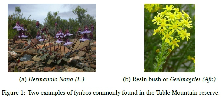
Generally speaking, the term 'fynbos' refers to vegetation dominated by evergreen woody shrubs with small and hard leaves that have a linear or needle-like shape (Van Wyk, 2000). It is understood by ecologists and botanists that 'fynbos' refers specifically to the distinctive sclerophyllous shrubland in the southwestern Cape of South Africa, particularly to species of the 'Cape Floristic Kingdom', which is the most varied of the plant kingdoms (Fraser & McMahon, 2004). In this paper, 'fynbos' refers to these types of plants.

Figure 1 illustrates two types of fynbos: on the left, the Hermannia Nana (L.) colloquially called the windpomp poprosie in Afrikaans, and on the right, the resin bush, or in Afrikaans the geelmagriet (Euryop Abrotanifolius (L.)). The windpomp poprosie has distinctive leaves that are broad with serrated ends, whereas the geelmagriet has a markedly different stem and leaf structure that is comprised of small and less distinctive leaves.

2.1 Current tools for identification of plants

Tools for the identification of plants from their leaves are generally based on identifying species prevalent in the northern hemisphere, particularly plants found in forest or thicket biomes (Van Wyk, 2000). These plant types, particularly tree leaves, usually have broader leaves with distinctive characteristics that help to identify the plant families (Williams, 2007). While many fynbos leaves do share similarities with northern hemisphere leaves, and although the same leaf classification methods could thus be applied, existing methods are ineffective for many types of fynbos. Existing online facilities for classification of plants using leaves tend to need human intervention: the user must first understand how to classify leaves and then do visual comparisons, working through a list of plant families and photos to identify the specific plant. An example of this is the Ohio Public Library Information Network's tree identification web guide, using the 'identify by leaf' option (OPLIN, 2013). Similar services, e.g. Project Noah (Networked Organisms, 2016) and the PlantzAfrica online dictionary (South African National Biodiversity Institute, 2016), are available to help identify and access information about fynbos and other South African plants, although users need to know the principles of identifying plants from their flowers or leaves to use these services.

2.2 How FLORA differs from existing tools for leaf-based plant recognition

Various automated image processing software tools are available to assist in classifying plants based on their leaves. The LEASYS program was developed for identifying certain Nigerian savanna trees (Abdulrahaman, Asaju, Arigbede, & Oladele, 2010) based on leaf morphology. LEASYS works by guiding the user through menu choices to narrow down the options of plants from which the leaf came.

FLORA differs from LEASYS in several ways: while LEASYS guides the user through a sequence of menus to identify leaves, FLORA aims to provide an automated way of loading a leaf photograph into the system; the photograph is then processed by automatic algorithms to suggest which plants may match the leaf. The advantage of LEAFSYS is that it is highly accurate; however the accuracy is limited by the user's ability to identify and differentiate specific plant features, and it also takes several minutes to identify a plant at a time. FLORA is intended as an automatic system that needs minimal user interaction besides taking and uploading photographs.

Leafsnap (Kumar et al., 2012) is a large collaborative project to develop a software tool to identify plant species from photographs. Initially focused on species in the U.S.A, the project has expanded to include trees from Canada and the United Kingdom. Users can use Leafsnap to upload photographs to a repository and can apply labels to potential matching plant names for the photographs. Photographs are taken of a single leaf on a white background, which is then processed by automatic algorithms. An internet connection is needed, as the processing operations are performed centrally; the processing takes approximately 6s, excluding time to photograph, upload images and display results. The application includes a field guide that users can browse off-line.

FLORA focuses on plant species in South Africa, mainly shrubs and fynbos plants of the CFK. FLORA models the shapes of the leaves by determining a collection of leaf descriptor features, which are computed using a series of image processing steps (explained in Section 4). Wu et al. (2007) developed a leaf recognition system, tested by using leaves from Jiangsu Sheng, China, that also determines leaf descriptors as part of the recognition process. It achieved an average prediction accuracy of 90.31% based on a database of 32 species, processing speed was not specified. Quadri and Sirshar (2015) used similar approaches to Wu et al. for extracting features and using a classifier to identify leaves. They achieved an accuracy of 100% but only using a dataset of 10 different leaf species, again processing speed was not specified. It achieved this using a Multi-Class Kernel Support Vector Machine classifier.

While the approaches used by Wu et al. have some similarities to methods used by FLORA, such as steps in preparing the leaf image, there are also many differences. For instance, Wu et al. use features such as diameter, physiological length, physiological width, and a probabilistic neural network to recognise leaves, whereas FLORA calculates a bounding ellipse and the convex hull of the leaf as features, which are then fed into a k-Nearest Neighbor (KNN) classifier to recognise the leaf.

2.3 Performance of the initial FLORA prototype, its limitations and revisions

The initial version of FLORA was developed as a rapid prototyped application using MATLAB. This initial version used only a database of thirteen leaves in the trials; it had an average prediction accuracy of 89.7%. It also had an average processing execution time of 9s for high-resolution images (3456 χ 2304 pixels) and 0.6s for low-resolution images (640 χ 400 pixels)(Winberg et al., 2013). The first version of FLORA has several limitations, particularly execution speed for high-resolution images and the lack of a modular code design.

This paper discusses two subsequent versions that were produced: FLORA-C and FLORA-G. FLORA-C was designed to be fast and standalone, depending on few (preferably no) other programs. FLORA-G was the GPU-accelerated version that extended FLORA-C, and was designed around accelerating image processing routines to improve performance.

2.4 General-purpose computing on graphics processing units (GPGPU)

GPGPU is the use of graphics processing units to carry out computations normally implemented on the CPU. A major advantage of using a GPU is its potential for highly parallelised computation that can provide a high throughput (Owens et al., 2008). However a drawback is that developing parallelised image processing routines for a GPU can be more challenging and time-consuming to code compared to writing equivalent sequential code (Munshi, Gaster, Mattson, Fung, & Ginsburg, 2011). An analysis done by Cook (2013) shows that, in some cases, a well-optimised CPU implementation may be more effective (in performance and/or development time) than a GPU implementation, depending on the type of operation performed.

Although there are architectural differences among GPU manufacturers, and even among the different models produced by the same manufacturer, the most modern GPUs share a similar architecture and programming model (Owens et al., 2008).

There are currently two major GPGPU platforms that are in wide use today and can be applied to the FLORA application, namely OpenCL and Compute Unified Device Architecture (CUDA).

OpenCL is the dominant open general-purpose GPU computing language, and is an open standard defined by the Khronos Group (Munshi et al., 2011). OpenCL is a framework for writing programs that can execute across multiple types of processing units including Central Processing Units (CPUs), Graphics Processing Units (GPUs), Digital Signal Processors (DSPs) and Field Programmable Gate Arrays (FPGAs), these are collectively referred to as 'compute devices'. Platforms that make use of more than one type of processing unit are generally referred to as 'heterogeneous computing platforms', GPGPU platforms can be considered as a specific type of heterogeneous computing platform in which only CPUs and GPUs are used.

CUDA is a proprietary parallel computing architecture and application program interface (API) created by Nvidia. It allows programmers to access low level capabilities of CUDA enabled graphics processing units in order to carry out general purpose computations (Cook, 2013). Programmers can have access to the CUDA platform through specially written libraries, compiler directives or through extensions of existing programming languages such as C++ and Fortran. CUDA also has support for the OpenCL standard. CUDA is currently one of the most widely used and mature GPGPU platforms used today since it is also one of the oldest.

2.5 GPU-based image processing for FLORA

CUDA was selected as the GPGPU platform for FLORA-G due to its mature code base and focus on acceleration using consumer GPUs specifically. We followed the generalised approach described by Owens et al. (2008) for developing and running CUDA kernels, which involves directly defining the computation domain as a structured array of threads, then creating a single SIMD (i.e., single instruction multiple data (Flynn, 2011)) function that is executed on GPU threads in parallel. A return value is computed for each thread using a combination of mathematical operations and memory access. The resultant data stored in global memory is then used as input for further computations or sent back to the CPU. A guide, including code examples, for implementing commonly used image processing routines is provided by Stava and Benes (2011), some of which we used in this project and have referred to in Section 4.

2.6 Leaf recognition techniques

FLORA as well as the other fully automatic leaf recognition applications mentioned in Section 2.2 make use of a number of image processing techniques in order to firstly separate the leaf shape from the image background and then identify or 'extract' unique features of the leaf that can be used with a statistical classifier to identify the plant species. This section will focus on the image processing and classification techniques used specifically by FLORA (and outlined in Figure 2). The first step, referred to as 'blob extraction' in FLORA, uses the following techniques: greyscale, Otsu threshold, region detection and image blur.

2.6.1 Greyscale

To grayscale an input image the red, green and blue values of each pixel were converted to a single greyscale intensity value that was written to the corresponding pixel in the output grayscale image. The greyscale values can be calculated using a weighted sum of RGB values as follows:

I_gray= 0.2989Ired + 0.5870I_green + 0.1140 I_blue

This equation is derived from CCIR 601 which is a standard for encoding analogue video signals in digital form, although other weightings may also be used (International Telecommunication Union, 1990).

2.6.2 Otsu threshold

Otsu thresholding (Zhang & Hu, 2008) works by splitting pixels of a greyscaled image into two classes: C₀(foreground) and C₁(background). The classes are separated by a threshold T such that pixels of class C₀have grey intensities in the range [1,2,... T ] and pixels of class C₁have grey intensities in the range [T + 1... L], where L is the maximum intensity value. In order to calculate the value of T, a grey level histogram is used; this histogram gives the distribution of the grey level intensities for pixels in the image. The histogram is computed by counting the number of pixels found of different intensity levels. A threshold value t is then calculated that minimizes the intra-class variance, defined as a weighted sum of the variances of the two classes

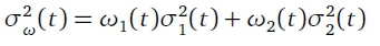
where ω_ι are the probabilities of the two classes, σ² the variances of the classes and t the threshold value. The threshold value t is calculated using an exhaustive search using all possible values of t. Once the Otsu value t = T was found a binary image is produced which contains only pixels with an intensity greater than or equal to T. Figure 5c shows an example of a binary image produced after Otsu thresholding.

2.6.3 Find image regions

Region detection involves checking the number of image regions or 'blobs' in a binary image. FLORA makes use of the Connected Component Labeling algorithm to achieve this (Stáva & Benes, 2011). Connected Component Labelling (CCL) is an algorithmic application of graph theory where sets of connected components are identified and labelled based on certain rules. In the case of FLORA's implementation, a region is defined as a group of non-zero pixels (white) that are surrounded by zero pixels (black).

2.6.4 Image blur

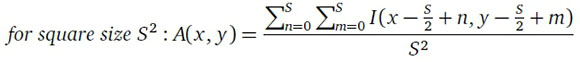
Image blurring can be achieved using a simple averaging filter. The averaging filter works by treating the image as a 2D matrix of integer values I(x, y) that represent the pixel intensities: the pixel intensity of each pixel in the image is then replaced with the average intensity of a square group of pixels of which the target pixel is the centre.

Other filters for blurring that can be used include the bilateral blur, Gaussian blur and median blur.

2.6.5 Feature extraction

Once the leaf shape is extracted leaf recognition applications make use of several unique leaf features in order to differentiate and identify particular species, FLORA uses the following: rectangularity, solidity, convex perimeter ratio and form factor (Winberg et al., 2013). Rectangularity is the ratio of the extracted region area to the area of the smallest bounding rectangle that fits the region, solidity is the ratio of the region area to the area of the convex hull that fits around the region, convex perimeter ratio is the ratio of the region perimeter to the perimeter of the convex hull and form factor is a ratio used to describe how similar the region area is to a circle, it is effectively the ratio of the region area to the perimeter squared.

2.6.6 Rotation and orientation

These features are however not all rotationally invariant and a rotation processing step is also included in the FLORA application to ensure leaf orientation does not affect prediction accuracy. Rotation can be achieved using a rotational matrix transform, where the coordinates of each pixel are transformed as follows:

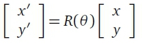
where (x, y) are the coordinates of the original pixel and (x', y') are the coordinates of the rotated pixel. R(θ) is the following transformation matrix:

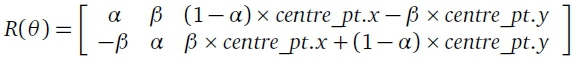
where a = cos(B) and β = sin(θ). This rotation matrix is used to rotate any set of 2D points θ degrees about the point centre_pt. For the FLORA implementation the centre_pt is defined to be the center of the input image since it is expected that the leaf region will be in the center of the image. The angle of rotation θ is calculated in FLORA using a method proposed by Chen (1990). This method involves calculations using image moments.

2.6.7 K-nearest neighbour classifier

Once image processing is complete a statistical classifier is used to either build or query a database to allow identification of plant species. FLORA makes use of the K-nearest neighbor classifier with the parameter K=1, this is also known as simply the nearest neighbor algorithm (Winberg et al., 2013). The algorithm works by creating an N dimensional feature space in which each of the N dimensions represents a particular feature. In the case of FLORA, four different features are used and thus the feature space has four dimensions. When building the database (also referred to as training the classifier), points are created in the 4D space using features extracted from previously classified images. When doing a prediction, the extracted features are used to create an input point in the 4D space, the Euclidean distance between the calculated input point and the other existing points in the database are then calculated. The point in the database with smallest Euclidean distance to the input point is then used to classify the input point.

 

3 METHODOLOGY

The methodology for developing FLORA-C and the subsequent FLORA-G followed a process whereby the initial prototype, previously developed as a rapid prototype using MATLAB, was redesigned as a C++ application then accelerated using GPU acceleration. FLORA-C implemented all the same processing functions as the original MATLAB version using C++ based libraries, there were no modifications to the original application design.

For the development of FLORA-G core image processing operations that prepared the leaf images for identification, and that took up much of the processing time, were converted into CUDA kernels to run on the GPU. Overall, the development followed these five steps:

• Step 1: code review and processing time analysis of the initial FLORA-C prototype.

• Step 2: investigation of related work, identifying tools and libraries for GPU acceleration, and acquisition of sample photographs for testing.

• Step 3: Identifying bottlenecks and aspects of the code that would benefit from being made parallel.

• Step 4: design and coding of GPU kernels to accelerate bottlenecks.

• Step 5: comprehensive performance analysis, comparing the different versions and checking that accuracy is maintained.

The first step involved reviewing and performance testing of the original MATLAB implementation to understand its operation and to identify bottlenecks of the computer vision algorithms for potential speed enhancement. The 'tic' and 'toc' MATLAB functions were used to measure the 'wall clock' execution times to microsecond accuracy of the identified processing routines in the MATLAB scripts.

The second step started with an investigation of the FLORA MATLAB code to review needed image processing methods and configurable parameters. During this stage, a literature review was done to investigate related research and to consider tools and libraries to use for developing a C++ version of the program. These insights guided the high-level design of FLORA-C (the C++ version of FLORA) which would serve as the foundation to FLORA-G, the GPU-accelerated version of FLORA for which the design is shown in Section 5. Leaf images were also collected during this step.

The third step involved implementing FLORA-C following the high-level design produced in step 2. This included porting the MATLAB scripts and toolkit function calls to equivalent, sequential, C++ code. FLORA-C was implemented as a standalone C++ program running under Microsoft Windows 7. The OpenCV 3.0.0 library was utilised for some of the image processing algorithms detailed in Section 4. The code was compiled using Microsoft Visual Studio 2013. During this step, processing bottlenecks were identified to determine which parts of the code took the longest to run and which could thus benefit from being converted into GPU kernels. The Microsoft Visual Studio 2013 profiler was used, in instrumentation mode, to measure execution times.

In the fourth step, image processing algorithms identified as bottlenecks were translated to run on a GPU (see Section 5). Some processing operations can be considerably difficult, or poorly suited, to make parallel and run on a GPU (Tristram & Bradshaw, 2014), therefore this stage included decisions on whether particular bottlenecks should be implemented on the GPU or not. The CUDA Development Toolkit v7.5 was chosen for implementing FLORA-G.

In the fifth step, performance benchmarking was done for FLORA-C and FLORA-G. Execution times for the C++ and the CUDA accelerated implementations were both found using the Microsoft Visual Studio 2013 profiler. The prediction accuracies between versions were also checked.

The different versions of FLORA were all tested using a PC running 64-bit Microsoft Windows 7 with a Intel i5-2320 processor, clocked at 3GHz, and 16GB RAM. An Nvidia GeForce GTX 550Ti GPU with 1GB video memory was used for running the CUDA kernels.

The photographs of the fynbos leaves were collected with permission from the Kirstenbosch botanical garden in Cape Town. Each photo was taken with a piece of white paper held behind the leaf to provide a clear background. The leaf photos were categorised manually, according to the label plaques next to the plants in Kirstenbosch or using Manning and Paterson-Jones's Field Guide to Fynbos (Manning & Paterson-Jones, 2007). Each plant entry in the database can link to one or more leaf photos and to a photo of the plant. Table 1 shows the leaf table of the database.

A total of thirteen fynbos species were photographed with ten photographs taken per species. Additional photographs (ten per species) of other plant species were also used, including four northern oak species and four northern maple species. These photos were taken from the Leafsnap dataset(Kumar et al., 2012). These extra photos were included to ensure the test dataset was statistically significant enough. The Plant ID (a sample number Sn in Table 1, which was assigned to each species of plant) was used as a key to allow the researchers to cross-reference each of the leaves in the database with their parent specimen, hence allowing information about the plant to which the leaf belongs to be easily obtainable.

3.1 Testing methodology

In order to determine the effectiveness of FLORA-C and FLORA-G it was required that the prediction accuracy and execution time be tested and compared to the original MATLAB implementation.

3.1.1 Prediction accuracy

Twenty-one species of plants were used, with photographs taken of 10 different leaves of each species. Leaf images of resolution 3456 χ 2304 pixels were used in all these tests. For each version of FLORA, the program was initially trained using seven out of the ten leaf photographs per species: this resulted in a classifier database with 147 entries total. The two tests described below were then performed for each version of FLORA.

For Test 1, the system was tested to see if it could correctly recognise the species of plant from a different leaf photograph from the one used to train the system for that species. The 63 images (three per species) that were not used to train the program were used for this test. The confidence level computed for each prediction was examined and an average of the confidence levels for correct predictions and for incorrect predictions was calculated, as well as the average prediction accuracy for valid input. The confidence measure for each match is set to one minus the distance between the potential leaf match and the input leaf, divided by the Euclidean distance of the most distant leaf match in the database. All 21 species that the system learned were tested.

Test 2 was performed to see how the program responds to leaves from species that it was not trained to recognize, i.e. to determine confidence levels of false positives. For Test 2, 30 leaf images were taken from plants that the system was not configured to recognise and tested. The application always returns a confidence level. It was expected that low confidence levels, below 50%, would be considered a rejection for the prediction result returned by the program. The average of the confidence measures from each of the 30 predictions was calculated. In total, six tests were done for prediction accuracy, i.e., Tests 1 and 2 were performed for each version of FLORA.

3.1.2 Execution speed-up

In order to determine the achieved speed-ups of FLORA-C and FLORA-G, the execution time performance of all FLORA implementations must be determined and compared. Execution time tests were done by carrying out predictions using 5 different leaf images of the same species. Images from the same species were used to help ensure that processing stages that may be carried out more than once, such as 'image blur' and 'Otsu threshold' (Figure 2), are carried out the same number of times. This was also confirmed explicitly.

During the prediction process each processing stage of the FLORA implementations (identified in Figure 2) was timed. The final execution times were then taken as the average of the times achieved in the five predictions: each leaf was processed once, as opposed to processing it twice and discarding the first reading. This was done to more closely match normal use. Using the final average execution times for each FLORA implementation, the speed-ups achieved in FLORA-C and FLORA-G could then be determined.

 

4 DESIGN OF FLORA-C

The processing steps used in the original FLORA application are shown in Figure 2. FLORA-C was developed to follow the same process. To reduce the development time of FLORA-C, and to ensure good performance, the initial C++ implementation of the processing algorithms used OpenCV libraries. The code was kept modular to make it easier to maintain and to allow for future reuse.

As seen in Figure 2, the processing stages (light blue blocks) are grouped into components of related functionality that work together, such as the feature extraction component that finds and extracts features from leaf images. Each operation is implemented in its own class within separate C++ code modules.

4.1 Leaf image preparation

Like the original MATLAB version of FLORA, the C++ implementation expects input images to contain only a single leaf on a white background. This helps to ensure that only the leaf region is extracted during processing.

Figure 5 illustrates the results of the processing stages carried out by the program. The source image, the leaf photograph to be identified, is first loaded into the program (Figure 5(a)) and then converted to grayscale (Figure 5(b)). The conversion to grayscale was performed by the CPU using the weighted sum method described in Section 2.6.

Otsu thresholding was then applied to separate the image foreground, i.e. the leaf of interest, and the background. Once separated, the background pixels were colored black and the foreground white. Once thresholding is complete the number of regions in the resulting image is determined using the Connected Component Labeling (CCL) algorithm. If the number of regions is greater than one an averaging filter (blur) is applied to the greyscale image and the Otsu threshold and CCL steps are repeated.

The next stage of the process involves rotating the leaf image so that its major axis lies parallel with the x-axis. This is achieved by first determining the angle of rotation using image moments and applying a rotational matrix transform, treating the input image as a matrix. Following rotation the input image is ready for feature extraction.

4.2 Feature extraction and prediction

First the leaf contour is extracted, followed by the convex hull and the bounding box. Available OpenCV libraries were used for these steps, examples of these features can be seen in Figure 5. These features are then used to calculate the four feature ratios used by FLORA - rectangularity, solidity, convex perimeter ratio and form factor - described in Section 2.6. The final step is to predict which plant the leaf came from. In development of the first version of FLORA a selection of classifiers were tested including probabilistic neural network, general regression neural networks and KNN algorithms (Winberg et al., 2013). Prediction using a KNN classifier with K = 1 provided the best results in the experiments and was therefore chosen for use in FLORA. OpenCV libraries were used for implementing the classifier in FLORA-C and FLORA-G.

 

5 DESIGN OF FLORA-G

The design of FLORA-G was initiated after the completion of FLORA-C. Following the methodology described in Section 3, design of FLORA-G started by identifying the most time consuming functions in FLORA-C that could then be accelerated. The execution time and prediction accuracy of FLORA-C was evaluated for both low resolution and high resolution in order to identify parts of the application that could benefit the most from GPU-acceleration. The most time-consuming functions were 'Otsu threshold', followed by 'Greyscale', 'Apply image rotation', and 'Find image regions'. GPU-accelerated versions of these functions were therefore developed. The final version of FLORA-G combined both non-accelerated C++ functions and GPU-accelerated functions, because only GPU-accelerated functions that were shown to yield performance improvements over the non-accelerated versions were kept in the application. Results showed (see Section 6.3) that prediction accuracy was unaffected by higher resolution images for the leaves tested but did result in higher execution time. Therefore the design of FLORA-G was optimised for lower resolution input.

5.1 Greyscale image

The 'load input image' function in FLORA-C is actually responsible for two functions, firstly it loads the input image into system memory and converts the image to greyscale, this is done at the same time in one operation.

In an attempt to accelerate this function it was rewritten to allow the input image to be loaded into GPU memory and the greyscale function to be carried out in parallel on the GPU. This was achieved using a simple GPU kernel that applies the weighted RGB formula described in Section 2.6 to every pixel in the input image in parallel threads. An available OpenCV CUDA accelerated library was used to implement this.

It was found however that the additional overhead required was too great to allow for any performance gains, it included first loading the input image in color to main memory, transferring the input image to GPU memory and then transferring the result back to main memory for the Otsu thresholding step. The original FLORA-C implementation of image loading and greyscale was therefore used as is for FLORA-G.

5.2 Otsu threshold

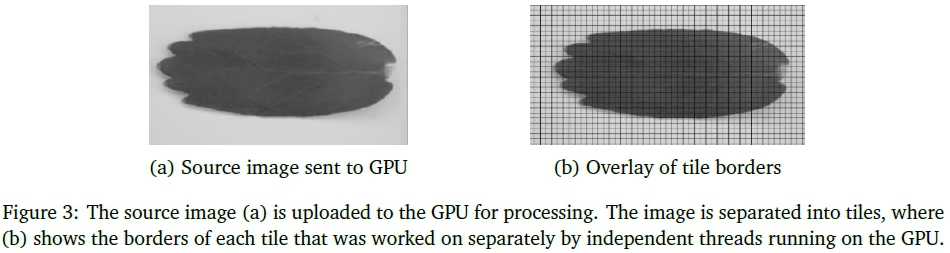
To accelerate the Otsu thresholding function it was implemented on the GPU using the approach proposed by Singh, Sharma, Mittal, and Ghosh (2011). First a grey level histogram was computed by counting the number of pixels found of different intensity levels; a kernel was loaded onto the GPU to perform this on the grayscale image that had been uploaded to the GPU. A 256-element array was created in the GPU memory to hold the resultant histogram. The image was divided up into a grid of pixel tiles, one tile for each thread (the number of threads being based on the cores available on the GPU). Figure 3 illustrates how the grayscale image was divided into tiles.

Each thread instantiated its own array in shared memory to produce a sub-histogram for its window, which was then merged with the resultant histogram in global memory. Once the histogram was complete, it was transferred to the main memory, where the CPU then normalised the histogram to treat it as a probability distribution.

An exhaustive search was then done on the CPU to find the Otsu value t using the calculated histogram. This was done on the CPU because FLORA was designed to use 8-bit greyscale, meaning that the grey level histogram is always 256 elements and the processing of this relatively small array has negligible performance impact. This threshold value was then sent to the GPU. A thresholding kernel was then implemented on the original greyscale image (still in GPU memory) to produce a binary (i.e. black and white) image that demarcated background and foreground pixels. Figure 5(c) shows the resultant binary image.

5.3 Apply image rotation

Application of image rotation takes place after image orientation has been determined. To implement image rotation on the GPU the same method of using a rotation matrix and matrix transform was used as in FLORA-C, however the matrix transform operation was applied on the GPU using an available OpenCV kernel that applied the matrix multiplication operation in parallel on all the pixels of the input image.

5.4 Find image contours

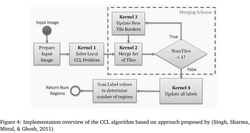
The process of finding image contours was performed by using the CCL algorithm described by Stáva and Benes (2011) to find a single foreground region. This algorithm was coded in C++ and CUDA libraries directly. The implementation followed the Parallel Union Find CCL variant of the CCL algorithm, as explained by Stáva and Benes. Figure 4 shows how four CUDA kernels were developed to implement this algorithm to work on a binarised input image.

The algorithm requires the image to be a square with sides a power of two in length; hence, a "prepare input image" step was first performed on the CPU to determine a suitable size. This step also allocated a 2D array of that size on the GPU to store an equivalence array: this was used to represent equivalence trees, whereby an element in the array stored an index of a pixel with an equivalent label. An element of the equivalence array equal to its own index corresponded to a root of an equivalence tree. Initially, each element of the equivalence array was initialised to its own index number (this starting point corresponds to the worst case state of no equivalence, i.e. no neighboring pixels of the same color).

Borders of the background color (black) were added to the image to get to a suitable size: these borders were implemented as a virtual window overlay such that whenever a kernel thread read a pixel in the border, the background color was returned.

The input image was divided into tiles of 8 χ 8 pixels each and distributed among the available GPU cores for execution of CCL kernel 1. This kernel applied the CCL algorithm each time that two neighboring foreground colored pixels in the 8x8 tile were found that did not share the same label. The kernel stopped once all the connected components in the local solution (i.e. the individual 8x8 tiles) were found. Next, kernels 2 and 3 were executed alternately. Kernel 2 merged sets of tiles into larger tiles. Kernel 3 flattened the equivalence trees between successive applications of kernel 2. Finally, kernel 4 ran, after the tiles had all been merged, to update all the labels; it placed these into a 2D label array (which mapped a label to each pixel of the input image). This array was sent to the CPU, which scanned the array to count the number of separate foreground regions in the image.

5.5 Extracting leaf descriptor features

Once the input leaf shape is extracted and rotated, feature extraction takes place. Firstly the region outline, bounding box and convex hull were determined. These features were then used to calculate the four feature descriptors used to predict which plant the leaf came from using a KNN classifier.

Once the input leaf shape is extracted and rotated, feature extraction takes place. Firstly, the region outline, bounding box and convex hull were determined. These features were then used to calculate the four feature descriptors used to predict which plant the leaf came from using a KNN classifier. The most time-consuming part of the feature extraction stage was calculating the convex hull, which only consumed on average 1.73% of the total execution time for FLORA-C using low resolution photos, and even less for high resolution.

All these steps combined only added up to 3.94% of the total execution time, amounting to 7.68ms on average for the large image sizes using FLORA-C. Therefore, it was decided these steps would not be implemented on the GPU due to the GPU overheads, such as additional system memory transfers, that would offset any potential performance gain.

The final step of FLORA's leaf recognition process is the KNN classifier. Like the feature extraction stage, the KNN classifier took a small portion of the overall execution time (specifically 0.13% on average for high resolution images) compared to other programming steps; it was therefore concluded that GPU acceleration of this stage would provide at best negligible performance gains.

However, it should be noted that this quick execution time is due to the small leaf database used. The time to run the KNN classifier is proportional to the database size considering that for larger databases more Euclidian distance calculations and comparisons would need to be done. GPU acceleration of the KNN classifier will therefore be investigated as future work.

 

6 PERFORMANCE RESULTS

To evaluate the performance of FLORA-C and FLORA-G the average execution time of each processing stage was determined and compared to the original MATLAB implementation.

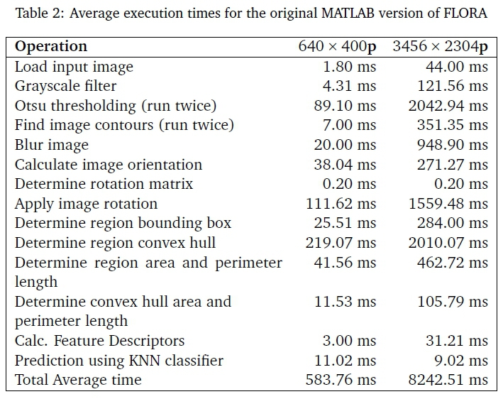
All FLORA implementations were tested using the methodology explained in Section 3.1. Table 2 shows the average execution times for each processing stage of the original MATLAB implementation for both 640 x 400 pixel input and 3456 x 2304 pixel input.

6.1 FLORA-C speed-up

Table 3 shows FLORA-C's average speed-up of processing each stage for low-resolution and high resolution images. FLORA-C executed much faster than the MATLAB prototype in all processing stages, completing execution of the low-resolution cases around 90 times faster than the MATLAB prototype. The speed-up was much less for high-resolution images however, with FLORA-C achieving a total average speed-up of only 42 compared to the MATLAB prototype.

This experiment shows that the conversion to C++ greatly improved the performance, but performance gains were reduced overall when using larger resolution input. The C++ operation that took the longest for low-resolution images was the Otsu threshold stage which took 17% of the execution time. In the case of high-resolution images, the finding of image contours (CCL) dominated the processing time, taking 23% of the total run time. The largest processing bottlenecks identified from multiple runs of FLORA-C were: Otsu thresholding (17%), Greyscale filter (17%), Apply image rotation (16%), and find image contours (11%).

It was found that the first time FLORA-C runs there is an additional fixed delay where initialising of OpenCV libraries takes place, this delay was excluded from speed-up calculations as it could be avoided by running the FLORA-C application as a continuous service rather than calling a new instance of the application for each prediction request. Including the initialisation delay, the total average speed-up of FLORA-C compared to the MATLAB prototype reduced to 2 χ for low resolution input and 18χ for high resolution images.

6.2 GPU-acceleration of FLORA-G

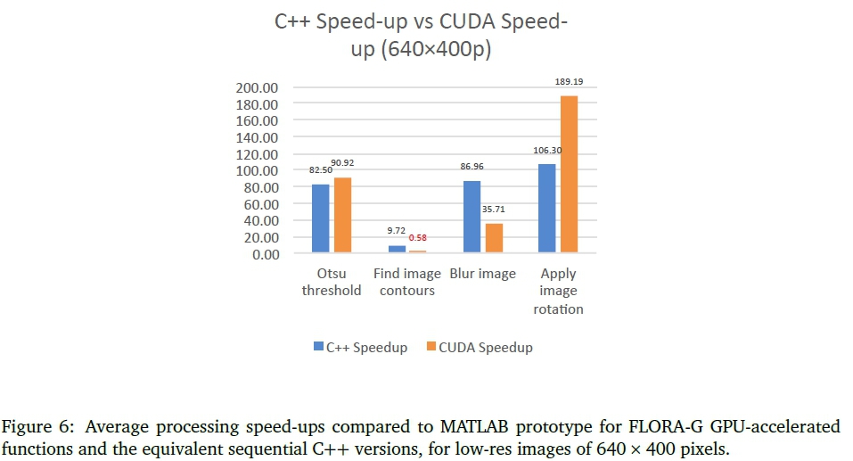
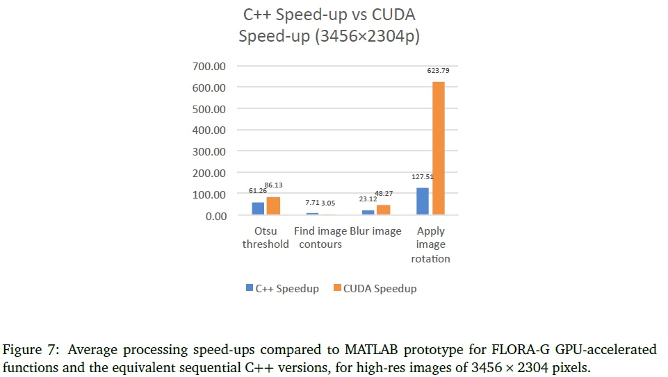
Performance differences between GPU-accelerated functions in FLORA-G and original C++ functions in FLORA-C are shown in Figures 6 and 7, showing results for low-resolution images (640 χ 400) and high-resolution images (3456 χ 2304) in terms of speed-up other the original MATLAB implementions (i.e. the values speed-up values for the C++ functions and for CUDA functions are relative to the functions run in the MATLAB version). As can be seen from Figure 6, FLORA-G performed poorly with low resolution images compared to FLORA-C, the only exception being the Otsu threshold function where the GPU-accelerated version performed slightly better. The worst performing GPU-accelerated function was the 'find image contours' which actually performed about two times slower than the original MATLAB version.

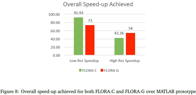
The overall speed-up achieved for both FLORA-C and FLORA-G over the MATLAB prototype is shown in Figure 8. The final version of FLORA-G only implemented the GPU-accelerated versions of 'Otsu threshold', 'Blur image' and Apply image rotation' as the GPU-accelerated 'Find image contours' function underperformed when using both low resolution and high resolution input.

As was the case with FLORA-C a fixed initialisation delay was observed when running FLORA-G for the first time, this delay was much larger however do to the additional overhead related to initialisation of the GPU (CUDA) libraries. With initialisation delays included, FLORA-G took twice as long to execute compared to the MATLAB version for the low resolution input and only managed a speed-up of 7x for high resolution input. Like in the case of FLORA-C this delay was not considered as it could be avoided by modifying the FLORA-G program to run as a continuous service rather than calling a new instance for every prediction.

6.3 Prediction accuracy testing

Prediction accuracy testing was performed to compare the accuracy of the different versions of FLORA, namely the original MATLAB prototype, FLORA-C and the FLORA-G. These tests were not done to gain a general sense of the program's prediction accuracy for a wide range of plants, but rather to check that revised versions of FLORA maintained similar prediction accuracies. The testing methodology is described in Section 3.1.1.

The results for Test 1 are summarised in Table 4, reporting how each version of FLORA performed for accuracy and showing the following characteristics for each test: number correct classifications, number misclassincations, average confidence level for correct classifications, and average confidence level for incorrect classifications. Table 5 shows the results for Test 2. Since all the images used in Test 2 were from plants not learned by the application, the results show the number of classifications that were predicted with a confidence below 50% and the number predicted with a confidence of 50% or more. The application always provides a prediction if the leaf database is not empty, and it returns a confidence level for each prediction. Therefore, for each leaf tested in Test 2, the prediction result was considered a success if the returned confidence level was below 50%, i.e. the application was not confident in predicting species not in its leaf database.

For Test 1, all versions of the program made exactly the same predictions in identifying from which plant the leaf images were. The original MATLAB version provided a slightly higher confidence level on average for matches performed, which can likely be attributed to the calculations being done at higher precision in MATLAB.

In performing tests with an image resolution of 640 χ 400 pixels, it was found that the prediction accuracy for these lower resolution images had a slightly lower confidence level than for higher resolutions images, although the same predictions were made. Nine leaves were misclassified in Test 1, and the same misclassincations happened in all versions of FLORA; a low confidence level of 41% was given for that leaf, despite the system having learned that species from a different leaf image from the same plant species.

In terms of testing leaves that the application had not learned, the resultant confidence level was below 50% for each leaf tested, which indicated the confidence calculation was working effectively as a means to suggest that an input leaf was not recognised by the system.

Overall, the prediction accuracy testing was considered successful, as there was little difference (not more than 1% change) between the average confidence measures calculated in the tests. Furthermore, the standard deviation between the confidence measures for correct predictions in Test 1 was less than 2% for all versions.

 

7 DISCUSSION AND CONCLUSIONS

The FLORA prototype was successfully implemented as a C++ application, and a selection of the image processing routines were converted to CUDAkernels to speed-up the processing. Both FLORA-C and the GPU-accelerated FLORA-G showed performance improvements compared to the earlier MATLAB prototype. For low-resolution 640 χ 400 images, FLORA-C achieved an overall average speed-up of 92χ over the original MATLAB prototype while FLORA-G achieved an average speed-up of 73χ, excluding program initialisation latencies. In the case of 3456 χ 2304 images, the speed-up was 42χ for FLORA-C, and FLORA-G had a speed-up of 54χ compared to the MATLAB prototype.

For both high and low-resolution images, the most time was saved in determining the convex hull region, this function also achieved the most noticeable speed-up in both cases. For high-resolution images, the CUDA kernels all outperformed the equivalent sequential routines with exception of the 'find image contours' function which was therefore excluded from the final FLORA-G program. For the high-resolution images, the GPU-accelerated FLORA-G achieved a speed-up of 1.28χ on average over FLORA-C, but for low resolution images FLORA-G took 1.26 times longer to run than the CPU-only FLORA-C. This slower performance can be attributed to the additional memory overhead incurred when using a GPU and the added complexity of implementing parallelised versions of sequential code this includes loading the kernel and sharing global data between threads. This was especially true of the 'find image contours' function which required 4 kernels to implement on the GPU and ultimately underperformed compared to the CPU optimised FLORA-C.

While an individual CPU core is often faster (in instructions per second) than a GPU core, it is expected that the many cores of a GPU would leverage more parallelism as the image size increases, which would overcoming the kernel initialisation latencies thus providing operation that is faster compared to a CPU-only solution (Ryoo et al., 2008). The data transfer from the host CPU to the GPU was 256000 floats for 640 χ 400 low-resolution images and 7962624 floats for 3456 χ 2304 images. For the low-resolution images, the transfers between CPU and GPU took on average 16% of the total execution time while the high-resolution images on average took only 4% of the total execution time.

Photos taken from mobile devices nowadays often have higher than 640 χ 400 resolution, frequently beyond 2560 χ 1536 (i.e., 3.9 megapixels), which provides reason to use GPU-accelerated image processing operations for FLORA. In the case of batch processing of multiple images, the GPU-accelerated solution also has merit, considering that it could save time when processing multiple images at a time. A likely batch processing operation would be using alternate algorithms to build collections of different leaf descriptors for a leaf database, which would involve reprocessing all the images in a leaf database.

Reflecting on the FLORA development experience, we found that it was beneficial to develop a MATLAB prototype first in order to experiment with establishing an effective solution to the automated leaf identification problem, a decision that is inspired by, and in this case agrees with, lessons learned from the literature (Gordon & Bieman, 1995). The way that MATLAB code can be expressed concisely, and especially its library of powerful functions, saved much time during the prototyping stage. Once the processing stages and techniques had been decided, the conversion to the C++ executable went smoothly, facilitated by the OpenCV library and its good documentation. A console-based application incorporating all the processing stages was completed in the planned timeframe, taking three months. The GPU acceleration aspect took longer than expected, however, taking closer to two months instead of one. Setting up and compiling kernels using the Nvidia CUDA Toolkit went smoothly, but a lengthy learning curve was experienced in writing kernel code to leverage the architecture effectively. The Nvidia online tutorials were especially beneficial in improving productivity; in hindsight, it would have been better to work through these first before translating our own sequential code into CUDA versions. The objectives to develop a standalone program and then accelerating its processing using a GPU were achieved.

Plans for taking the FLORA application further include testing the system with a wider range of plant species and more leaf images per species; further code optimization, particularly of Otsu thresholding and convex hull calculation; and finally GPU acceleration of the KNN algorithm, for use when a large training database has been developed.

 

References

Abdulrahaman, A., Asaju, I. B., Arigbede, M. O., & Oladele, F. A. (2010). Computerized system for identification of some savanna tree species in Nigeria. Journal of Horticulture and Forestry, 2(6), 112-116.         [ Links ]

Chen, K. (1990). Efficient parallel algorithms for the computation of two-dimensional image moments. Pattern Recognition, 23(1-2), 109-119. https://doi.org/10.1016/0031-3203(90)90053-N        [ Links ]

Cook, S. (2013). CUDA Programming. CUDA Programming, (June), 441-502. https://doi.org/10.1016/B978-0-12-415933-4.00010-7

Flynn, M. (2011). Flynn's Taxonomy. In D. Padua (Ed.), Encyclopedia of parallel computing (pp. 689697). Boston, MA: Springer US. https://doi.org/10.1007/978-0-387-09766-4_2        [ Links ]

Fraser, M. & McMahon, L. (2004). A Fynbos Year. David Phillips Publishers.

Gordon, V S. & Bieman, J. M. (1995, January). Rapid prototyping: Lessons learned. IEEE Software, 12(1), 85-95. https://doi.org/10.1109/52.363162        [ Links ]

Harris, M. (2005). GPGPU: General-Purpose Computation on GPU. In Game Developers Conference (p. 30). San Fransisco: Nvidia Corporation.         [ Links ]

International Telecommunication Union. (1990). CCIR Rec. 601-2. Recommendations of the CCIR, 11 part 1 , 95-104.

Kumar, N., Belhumeur, P. N., Biswas, A., Jacobs, D. W., Kress, W. J., Lopez, I. C., & Soares, J. V. B. (2012). Leafsnap: A computer vision system for automatic plant species identification. In Computer vision-ECCV2012 (pp. 502-516). Springer. https://doi.org/10.1007/978-3-642-33709-3_36

Machanick, P (2015, December). How General-Purpose can a GPU be? South African Computer Journal, (57). https://doi.org/10.18489/sacj.v0i57.347

Manning, J. & Paterson-Jones, C. (2007). Field Guide to Fynbos. Cape Town: Struik.         [ Links ]

Munshi, A., Gaster, B., Mattson, T. G., Fung, J., & Ginsburg, D. (2011). The OpenCL 1.1 Language and API. In OpenCL programming guide (Chap. 1, pp. 1-83). Addison-Wesley Professional. https://doi.org/10.1109/SIPS.2009.5336267

Networked Organisms. (2016). Project Noah. Retrieved June 5,2016, from http://www.projectnoah.org/

OPLIN. (2013). What tree is it - identify by leaf. Retrieved December 23, 2013, from http://www.oplin.org/tree/leaf/byleaf.html

Owens, J. D., Houston, M., Luebke, D., Green, S., Stone, J. E., & Phillips, J. C. (2008). GPU Computing. Proceedings of the IEEE, 96(5), 879-899. https://doi.org/10.1109/JPROC.2008.917757        [ Links ]

Quadri, A. T. & Sirshar, M. (2015). Leaf recognition system using multi-class kernel support vector machine. International Journal ofComputer and Communication System Engineering, 2(2), 260-263.         [ Links ]

Ryoo, S., Rodrigues, C. I., Baghsorkhi, S. S., Stone, S. S., Kirk, D. B., & Hwu, W.-m. W. (2008). Optimization principles and application performance evaluation of a multithreaded GPU using CUDA. In Proceedings of the 13th ACM SIGPLAN Symposium on Principles and practice of parallel programming (pp. 73-82). ACM. https://doi.org/10.1145/1345206.1345220

Singh, B. M., Sharma, R., Mittal, A., & Ghosh, D. (2011). Parallel Implementation of Otsu's Binarization Approach on GPU. International Journal ofComputer Applications, 32(2), 16-21. https://doi.org/10.5120/3876-5417        [ Links ]

South African National Biodiversity Institute. (2016). PlantzAfrica. Retrieved June 8, 2016, from http://pza.sanbi.org/

Stava, O. & Benes, B. (2011). GPU Computing Gems Emerald Edition. Elsevier. https://doi.org/10.1016/B978-0-12-384988-5.00035-8

Stáva, O. & Benes, B. (2011). Connected component labeling in CUDA. GPU Computing Gems Emerald Edition, 569-581. https://doi.org/10.1016/B978-0-12-384988-5.00035-8

Tristram, D. & Bradshaw, K. (2014). Identifying attributes of GPU programs for difficulty evaluation. South African Computer Journal, 53. https://doi.org/10.18489/sacj.v53i0.195

Van Wyk, B. (2000). A photographic guide to wild flowers of South Africa. Struik.

Williams, M. D. (2007). Identifying trees: an all-season guide to eastern North America. Mechanicsburg, PA: Stackpole Books.         [ Links ]

Winberg, S., Katz, S., & Mishra, A. K. (2013). Fynbos leaf online plant recognition application. In Computer Vision, Pattern Recognition, Image Processing and Graphics (NCVPRIPG), 2013 Fourth National Conference on (pp. 1-4). IEEE. https://doi.org/10.1109/NCVPRIPG.2013.6776220

Wu, S. G., Bao, F. S., Xu, E. Y., Wang, Y.-X., Chang, Y.-F., & Xiang, Q.-L. (2007). A leaf recognition algorithm for plant classification using probabilistic neural network. In Signal Processing and Information Technology, 2007 IEEE International Symposium on (pp. 11-16). IEEE. https://doi.org/10.1109/ISSPIT.2007.4458016

Zhang, J. & Hu, J. (2008). Image Segmentation Based on 2D Otsu Method with Histogram Analysis. 2008 International Conference on Computer Science and Software Engineering, (1), 105-108. https://doi.org/10.1109/CSSE.2008.206        [ Links ]

 

 

Received: 11 Nov 2016
Accepted: 31 Oct 2017
Available online: 8 Dec 2017