Design of a Test Setup for Measuring all Load Components Acting on Tillage and Planting Implements

 

 

J. W. van Santen^I; C. J. Coetzee^II

^IDepartment of Mechanical and Mechatronic Engineering, University of Stellenbosch, South Africa
^IIDepartment of Mechanical and Mechatronic Engineering, University of Stellenbosch, South Africa. Email: ccoetzee@sun.ac.za

 

 

---

ABSTRACT

This project entailed the design, manufacture, and testing of a test setup with the ability to measure all load components acting on tillage and planting implements. In future, data obtained with the test setup can be used to perform accurate design calculations, as input into finite element simulations, and to perform accurate fatigue analysis. The design of implements can therefore be improved to better withstand the loads under various operational conditions and to minimise fatigue cracking. Laboratory controlled testing, and subsequent field tests, proved that the designed test setup was able to isolate and accurately measure each of the three orthogonal load components, as well as the main moment. It was further shown that the remaining two moments could be accurately calculated using the measured load components and fixed geometric lengths. The conclusion was drawn, based on field tests, that an increase in speed with the tine ripper had no significant effect on the mean load. Further, an increase in the working depth, resulted in an increase in the load, especially in the draught and vertical directions. Finally, it was shown that a decrease in turning radius (a tighter turn), resulted in an increase in the lateral force component.

Additional keywords: Agriculture, load measurement, tillage implements, planting, seeding

---

 

 

1 Introduction

Feeding the world population sustainably is becoming increasingly challenging, forcing the scale of farming operations to increase, in order to keep up with growing demand [1]. Field crops in South Africa contributed 25.8 % towards the gross value of the country's agricultural production in 2016/17 [2]. Larger and more sophisticated tillage-, seeding- and planting implements are needed by farmers to supply in the demand.

One of South Africa's leading manufacturers of seeding and planting implements is constantly trying to improve their designs an minimise down-time due to equipment breakdowns. A problem they are experiencing, is the development of fatigue cracks on the frames of their implements. To address this, further research into the exact cause of the problem is needed.

Designing implement frames to withstand various operational conditions, requires the load components acting on the implement to be known. This project entailed the design, manufacture, and testing of a test setup with the ability to measure all the load components acting on tillage and planting implements. In future, data obtained with the test setup can be used to perform accurate design calculations, it can be used as input into finite element models and used to perform accurate fatigue analysis. The design of implements can therefore be improved to withstand the operational loads and to minimize fatigue cracking.

 

1. Existing Test Setups

Although limited, experimental test setups to measure the force components acting on tillage tools exist. However, as far as the authors are aware, no such setup is commercially available, but designed and used by researchers to suit their specific needs.

Extended octagonal ring (EOR) drawbar transducers are used to measure the load exerted on the tractor's drawbar by a trailed implement. The measurement capabilities are either bi-axial (draught and vertical components), or triaxial (draught, vertical, and lateral components) and do not include moments [3,4]. EOR transducers can be complex to manufacture and could be susceptible to damage if not properly protected, as reported by [5] where an EOR was damaged and had to be replaced by a load cell system.

On the other hand, three-point hitch transducers are used to measure the force components acting on an implement which is attached to the tractor's three-point hitch system. Examples include the mounting of a transducer between the tractor and the implement [6] or measuring the loads in the links of the hitch system [7]. In the studies by [6,7] only the draught and vertical components could be measured, and not the lateral component or the moments.

A system where all three orthogonal force components and their relative moments could be measured, was designed by [8]. A series of four frames was connected to the three-point hitch system and each frame was restricted to have only a single degree-of-freedom relative to the previous frame. Load cells were used to measure the force for each degree-of-freedom. However, with the setup attached to the tractor's three-point hitch system, it could not simulate the behaviour of a trailed implement, such as those investigated in this study. The forces acting on a trailed implement are different to that of a hitched implement when the tractor turns for example, given the turning radius. Besides the difference in lateral displacement of the implement at the point of contact with the soil, trailed implements might also experience lateral wheel slip, further affecting the forces.

 

2 Test Setup Design and Layout

The final design of the test setup, as shown in figure 1, utilised a series of frames. The concept was based on that of [8], but instead of being attached to the three-point hitch system, the main frame formed a trailer to simulate drawn implements. With the frames connected to one another via linear bearings and load cells, it enabled each frame to translate or rotate in only one direction (degree-of-freedom) relative to the frame it is attached to. All the other degrees-of-freedom were eliminated by the linear bearings. The linear bearings were manufactured in-house, using diameter 40 mm stainless steel shafts and Vesconite bushes. The tolerance between the shaft and the bush varied between 0.001 mm and 0.002 mm.

The frames were constructed by welding square tubing (100 mm x 100 mm, 10 mm wall thickness) together and machining flat surfaces on the faces where the linear bearings were bolted onto.

The first frame was the main frame and attach to the tractor via the drawbar. Two wheels were attached to the rear of the frame and were height adjustable with the use of two hydraulic cylinders. The hydraulic cylinders controlled the respective actions of lowering the implement into and lifting it out of the soil.

A tine ripper unit was used for testing (a wide range of other units used for planting and/or seeding can also be attached). The ripper unit utilised a hydraulic cylinder to allow breakaway when a set force was experienced, protecting the unit from potential damage. A hydraulic accumulator was therefore needed as part of the hydraulic system on the test setup.

A cable extension position sensor was used to measure the angle between the tractor and the test setup (trailer). The position sensor measured linear displacement, but by placing the cable at an angle, triangulation could be used to calculate the angle, and thus the turning radius of the tractor.

A data acquisition system was housed in an enclosure and mounted on the main frame. Trailer lights were also installed to allow for safe road travel between testing locations.

 

3 Direct Measurement of Load Components

The test setup was capable of directly measuring the three orthogonal forces (draught, vertical and lateral), as well as the main moment component (due to the draught and vertical force components). The remaining two moment components could be calculated during post processing, using measurement data of the position of the tine (to account for breakaway). This assumed that the lateral force's application point on the tine, was the same as that of the main draught force and vertical force. This assumption was valid, since the maximum working depth of the tine with the knife point shear was only 187 mm. The draught force component is exerted on the frontal face/edge of the tool as a distributed pressure. Similarly, the lateral force component is distributed over the side face of the tool. With the upper layer (approximately 50 mm) of soil already loose, the distributed draught and lateral force components act over a length of approximately 140 mm measured from the bottom tip of the tool, with the effective point of application between 20 % and 35 % of this measurement [9], i.e., approximately 28 mm to 49 mm from the tip. On the other hand, the majority of the vertical force component acts close to the tip of the tool, where the tool meets the unbroken soil. The relative distance of 28 mm to 49 mm is small in comparison to the moment arm (Ly ~ 750 mm), and therefore it is assumed that the effective application point of the vertical and lateral force components is identical to that of the draught component.

The load cells measured a positive value in compression and a negative value in tension. Thus, when a draught force Fx was applied in the direction as shown in figure 2, Load Cell 1 would be in tension, resulting in a negative value. Since the draught force load cell would mostly experience tension during field tests, the positive axis was chosen in the direction of tension.

3.1Draught Force - Fx

The second frame was attached to the main frame (Frame 1) with the use of four linear bearings, figure 2. The linear bearings allowed for movement in only the horizontal direction. This movement was restricted with the use of a load cell (Load Cell 1, HBM U2B, 200 kN) attached to the front of the second frame and connected to a bracket that was attached to the main frame. Since movement in only the horizontal direction was allowed, the draught force Fx could thus be isolated and measured.

3.2Lateral Force - Fz

The third frame was attached to the second frame with the use of four linear bearings (figure 3). The linear bearings allowed for movement in only the lateral direction. A load cell (Load Cell 2, HBM U2B, 100 kN) between the second and third frame restricted the movement in the lateral direction and since the lateral force F_zwas isolated by the linear bearings, it could be measured by the load cell.

3.3Vertical Force - Fy

The fourth frame was connected to the third with four linear bearings allowing for movement in the vertical direction. This movement was restricted by two load cells (Load Cell 3a and 3b, HBM U2A, 20 kN), located on opposite corners of the fourth frame. The isolated vertical load Fy was then measured by the two load cells. Two load cells, diagonally opposite to each other, were used to help prevent tilting of the frame (around the x- and z-axis) due to forces applied at an offset, which induced a moment. A diagram of the configuration is shown in figure 4.

 

 

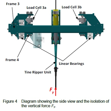
The diagonal positioning of the load cells allowed for the cancellation of moments created by both the draught and lateral forces. When a moment was induced on the vertical frame, one load cell would be in compression and the other in tension. The forces measured with the load cells should theoretically be equal in magnitude, but opposite in direction and thus cancelling each other out. The difference in measurement would therefore be the vertical load component.

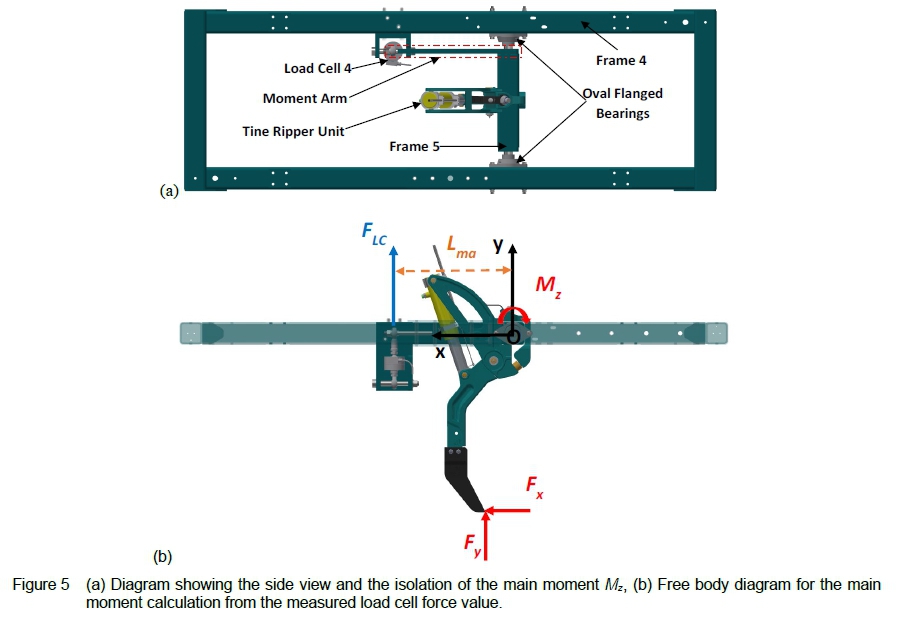
3.4 Main Moment - Mz

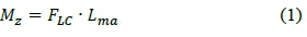
The fifth frame was attached to the fourth with two oval flanged pillow block bearings, allowing the frame to pivot around the center axis (figure 5a). The implement, in this case a tine ripper unit, was bolted to the fifth frame. A moment arm extended from the tubing of the fifth frame and had a load cell (Load Cell 4, HBM U2B, 20 kN) connected to its end, which in turn was attached to the fourth frame by means of a bolted bracket. The force measured by this load cell was due to the moment M_zcaused by the draught and vertical forces applied at an offset to the pivot of the fifth frame. The force Flc measured by the load cell was at a distance L_mafrom the pivot, as shown in figure 5b. The moment component M_z could therefore be calculated as follow,

 

4 Remaining Load Components

Since the draught, vertical and lateral forces were measured and the profile of the tine was known, the exact location (effective point of application) of the resultant force could be determined and the remaining two moments calculated.

4.1 Main Moment Mz Calculation

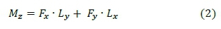
The main moment, due to the draught and vertical force components, acted around the z-axis. The origin of the coordinate system was located at point O as shown in figure 6. Ly is the vertical distance from the resultant force position to the origin, while L_xis the horizontal distance from the resultant force position to the origin. The main moment M_z was calculated by taking the sum of moments around the origin,

 

 

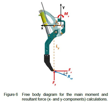
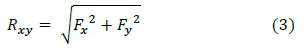
4.2 Resultant Force Rxy Magnitude and Direction

The draught F_xand vertical Fy force components were directly measured by the load cells. For each time stamp, the resultant force Rxy, due to these two components, was calculated,

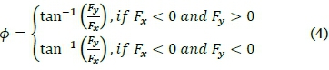
The angle of this resultant force with the horizontal (x-axis) was also calculated,

4.3 Application Point of the Resultant Force ^Rxy

A linear variable differential transformer (LVDT) was mounted on the hydraulic cylinder of the tine unit, as shown in figure 7a, to determine the exact position of the tine at any given point in time. This was used to accurately determine the resultant force's point of application on the tine.

 

 

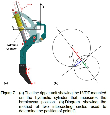
For each recorded data point, the LVDT measurement was used to calculate the coordinates of key points on the tine with reference to a global coordinate system with its origin at the tine's main pivot (labelled A in figure 7a). A MATLAB script was developed to process the recorded measurement data using the approach discussed below.

Points A, B and C form triangle ABC. Two lengths of ABC, i.e., AB and AC, remain constant as the tine pivots during breakaway. Points A and B are fixed, whilst the coordinates of point C are determined by the length BC (the length measured by the LVDT).

Figure 7b illustrates the method of two intersecting circles used to determine the position of point C. The first circle is drawn with its origin at point A and point C coincident on the diameter of the circle. A second circle is drawn with its origin at point B and point C coincident on the diameter. Points A, C and P form right triangle ACP and points B, C and P form the second right triangle BCP. The distance between the center of the circle can be defined as the sum of lengths a and b,

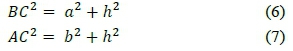
Using the Pythagorean theorem with triangles ACP and BCP, the following equations can be derived,

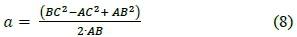
With the use of equation (5), a can be solved,

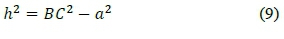
Solve for h by substituting equation (8) into equation (6),

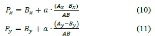
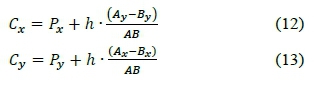
The x- and y-coordinates of point P can then be determined,

Finally, the coordinates of point C can be derived,

Once the position of point C is known, the coordinates of points U, S, and T can be determined using points A and C and the method of intersecting circles with each respective point.

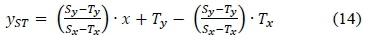
With all the moving coordinates on the tine known, the resultant force's application point could then be determined. The first step was to derive a straight-line equation for line ST, using the coordinates of points S and T,

When no breakaway was experienced, line US would be vertical and would have a fixed x-value, with the y-value varying between Uy and S_y. However, as soon as breakaway occurred, an equation for line US could be derived,

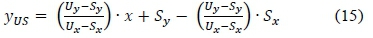
For each recorded data point, the constants in equations (14) and (17) were calculated using the LVDT measurement and method of intersecting circles. Starting at point T, and using increments of 0.01 mm, the candidate point of application was incremented along the lines ST and US. For each candidate point, the moment due to the two recorded force components F_xand Fy was calculated using equation (2). Once the moment was known for all candidate points, the final point of application was found by comparing the calculated moment to the measured moment (derived from equation (1)) and selecting the point which minimised the error. Note that for a breakaway angle of approximately 27°, the line ST became vertical, and equation (14) could no longer be applied. However, the coordinates on this vertical line were easily found.

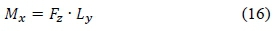
4.4 Moment around the x-Axis - Mx

With the resultant force's point of application known (section 5.3) and the vertical distance Ly therefore defined, the moment acting around the x-axis Mx was calculated using the measured lateral force F_z,

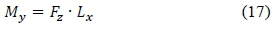
4.5 Moment around the y-Axis - My

The moment acting around the y-axis My could be calculated once the resultant force position was known (section 5.3) and the horizontal distance L_xtherefore defined. Using the measured lateral force F_z, My was calculated,

 

5 Laboratory Controlled Testing

Testing of the test setup was performed in a controlled environment to understand how the test setup performed when known load components were applied. The load cells were calibrated before testing to ensure accurate load measurement. These calibrations were performed before the load cells were installed on the test setup.

5.1 Load Cell Calibration

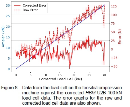
All the HBM load cells used on the test setup were new and never used before. Each load cell came with HBM's factory calibration sheet. They were however stored for several years, and it was therefore decided to perform calibration tests using a universal tensile/compression machine.

The factory calibration sheet was used for each load cell during the calibration tests and the data compared to the reading of the load cell on the tensile/compression machine. In figure 8, the maximum error/difference between the two load cells on a 30 kN load, is shown to be approximately 125 N (0.417 % and within the load cell accuracy). The calibration data of the other load cells showed similar results. The calibration tests proved that the factory calibration data of the load cells could still be considered trustworthy and were therefore used for each respective load cell on the test setup.

 

 

5.2 Experimental Setup

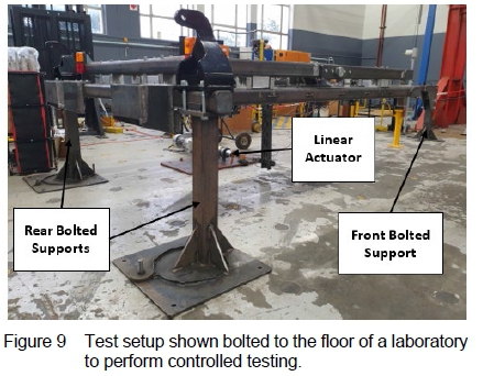
The test setup was held stationary by means of three specially designed supports that were bolted to the floor of the laboratory. One support was attached at the front of the test setup where the hitch is located and two supports at the rear wheel attachment locations, figure 9.

 

 

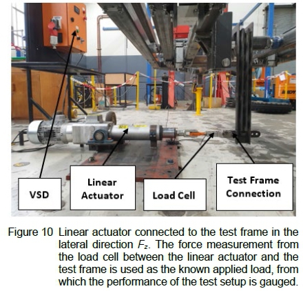
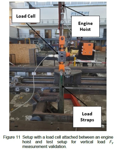
A Mecvel EC5 linear actuator, with a maximum force of 50 kN and stroke of 300 mm [10] was attached to a purposely designed mount which was bolted to the floor of the laboratory. An HBM S9 (50 kN) load cell was placed between the actuator and the frame of the test setup to measure the applied force, as shown in figure 10. The actuator was driven by a variable speed drive (VSD), allowing for precise control of the speed in both the draught and lateral force directions. For the vertical direction, a load cell attached to an engine hoist was used, where the load cell was connected with two load straps and D-shackles to the test setup, figure 11.

 

 

 

 

5.3 Results

Figure 12 shows the applied force from the linear actuator versus the measured draught force Fx on the test setup, for a typical test. The profile of the applied force was followed acceptably well by the load cell on the test frame. However, a slight lag was observed between the two profiles. This could be attributed to the effect of friction in the linear bearings. The frame isolating the draught force (Frame 2) carried the weight of all the other frames and components. The more weight, the larger the friction force would be.

 

 

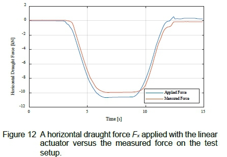
The mean difference in the applied and measured forces was calculated over the whole loading-unloading sequence. The test was then repeated 10 times, and the average difference was 0.7 kN (standard deviation 0.02 kN). This difference in force was close to the theoretical friction force of the bearing material, with Vesconite having a friction coefficient of 0.08 - 0.12, and the total mass supported by the four bearings being approximately 900 kg. A friction force of 0.7 kN would therefore equate to a friction coefficient of 0.08, which was within the design range. This means that the linear bearings performed as designed.

Furthermore, the correlation coefficient during loading (0 to 8 seconds) was 0.9985, with the coefficient of determination (R²) being 0.9970. The correlation coefficient during unloading (9 to 15 seconds) was 0.9963, with the coefficient of determination (R²) being 0.9926. The R² values achieved exceeded 0.99 and were therefore an indication of the high precision achieved with the test setup.

During field testing, the alternating loads from the soil and the wheel moving over uneven terrain would induce vibration on the entire test frame. To simulate what the effect of such a vibration on the force measurement would be, the frame was lightly struck by a hammer while the draught force was applied. These results are shown in figure 13. The profile of the applied force was followed noticeably closer by the load cell on the test frame when a vibration was present. The mean difference in the applied and measured force, was approximately 0.15 kN (reduced from 0.7 kN). Literature [11] shows that vibration can reduce the effects of friction, and this qualitative test (hammering) showed that during field testing, one can expect the frictional effects to be reduced, leading to even more accurate results.

 

 

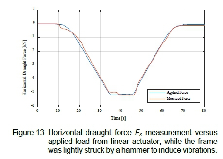
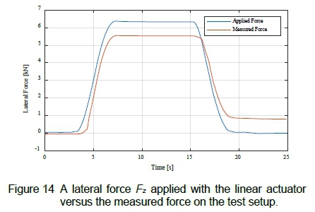
Figure 14 shows the applied force from the linear actuator versus the measured lateral force F_zon the test setup. The measured force closely followed the profile of the applied force, taking the effect of friction into account. The mean difference in measurement, between the applied and measured force, was approximately 0.68 kN. The linear bearings of Frame 3 carry a total mass of around 650 kg. This equates to a friction coefficient of 0.11. Though still within the design range, the friction coefficient obtained was higher than that of Frame 2. Several reasons for this are possible. One reason could be a rougher surface finish of the linear bearing shaft or bushing. Since these linear bearings were manufactured in-house, guaranteeing a consistent surface finish throughout was difficult. Another possible reason is slight misalignment of the frames and bearings. A slight misalignment would cause the shaft of the linear bearing to pinch within the bushing, increasing the friction. Like the testing of the draught force, the frame was lightly struck with a hammer to induce vibrations while testing. These vibrations showed favourable results in reducing the friction effects.

 

 

Testing of the test setup's vertical load measurement capability showed favourable results, figure 15. The profile of the applied force was closely followed by the load cell measurement on the test frame. The mean measurement difference between the applied- and measured force for the loading period shown, was approximately 0.14 kN. Given the magnitude of the total force, this difference was considered negligible.

 

 

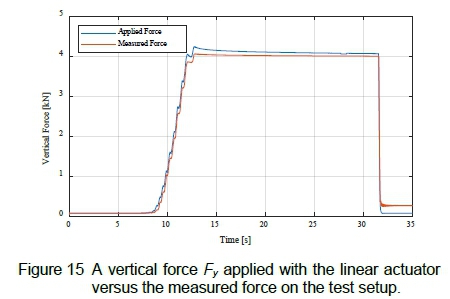
The load induced by the engine hoist was released by means of a hydraulic valve, releasing the hydraulic pressure in the lifting cylinder. The load release was almost instantaneous, causing the sudden drop shown in the graph. A 0.2 kN difference is observed in the measurements after the load was released. This could be attributed to friction forces inside the linear bearings preventing the linear frame from fully returning to its original position. The vibrations caused by the soil during field tests would minimise this effect.

 

6 Field Tests

The field tests were performed on a farm in the Boland region of the Western Cape, South Africa. The soil of the test area was a mixture of sandy loam and clay. Annual crops such as wheat and canola are typically grown in the area, as well as long term crops such as grapes and citrus.

6.1 Experimental Setup

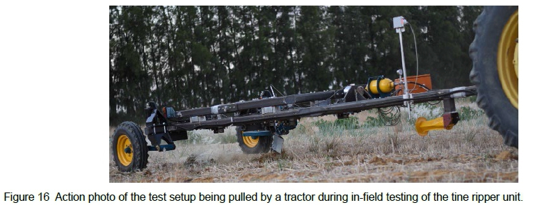
Figure 16 shows the test setup being towed by a tractor during in-field testing of the tine ripper unit. A comprehensive illustration of the test setup components is shown in figure 1. The test setup attached to the tractor's drawbar through a hitch and pin. The hydraulic hoses for the lifting and lowering of the test setup, as well as the charging of the accumulator, connected to the selective control valves (SCV's) of the tractor. The hydraulic systems could then be controlled from the tractor's cab using the SCV-remotes. A cable extension position sensor was mounted on the test frame and the cable attached to the centre of the tractor. As the tractor turned relative to the test setup, the distance measured with the position sensor changed, allowing the angle between the tractor and test setup to be determined.

The data acquisition (DAQ) system, comprised of two HBM QuantumX MX840B data loggers [12], was stored inside an enclosure mounted to the test setup's frame. The DAQ system was powered from the tractor's 12 V battery system through a 600 W pure sine-wave inverter. An electrical extension cable was run from the inverter to the DAQ system enclosure. The DAQ system was connected to a computer inside the tractor's cab, through a network cable. This enabled the load measurements to be observed live while the tests were in progress.

A GoPro video camera was also mounted on the test setup with a side-view of the tine ripper unit. Using a smartphone 'connected to the GoPro, the live video feed could be seen from the tractor's cab whilst testing was in progress. The video recordings of the test were used during post-processing to visualize the load measurements by synchronising the video to the measured data. This was done using HBM's CATMAN software where an offset could be placed on the video recording to match the timeframe of the measured data. The offset was determined by striking the tine with a hammer while the DAQ system was recording. The spike measured by the strain gauges on the tine (as discussed in the following section) and/or the load cell on the moment arm of Frame 5, was then matched to the time in the video of when the tine was struck.

For speed measurements, a handheld GPS unit (Garmin eTrex) was used. The tractor operator constantly monitored the GPS to ensure that the tractor speed remained at the set value.

6.2 Direct Frequency Measurement

Strain gauges, in a full Wheatstone bridge configuration for bending, were installed on the shank of the tine, just above the shear, as shown in figure 17.

 

 

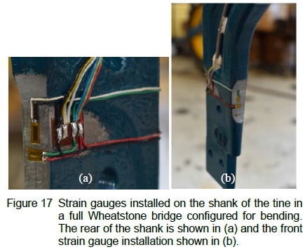
These strain gauges were the first point of measurement away from the contact interaction with the soil. Using a Fast Fourier Transform (FFT), the frequencies obtained from the strain gauge measurement was considered as the direct and actual frequencies induced on the ripper by the soil. These frequencies were then used as a reference during data processing.

Due to the elasticity of the test frames and linear bearings, slightly higher frequency data, compared to the frequencies measured by the strain gauges, could be observed in the data from the load cells. Using the highest frequency of 30 Hz measured by the strain gauges as reference, all frequencies in the load cell data higher than this reference value, were filtered out by applying a low-pass filter.

In future, the strain gauge measured frequency could also be a useful input for fatigue software analysis to further improve designs.

6.3 Data Sampling Rate

An appropriate frequency for data sampling had to be determined. The sampling rate and the speed of travel were dependent on each other, as shown in table 1. A sampling rate that was too low, would result in peak measurements to be omitted, due the nature of testing in a non-homogeneous medium such as soil.

 

 

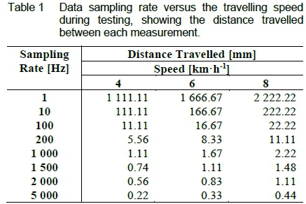
Soil conditions and composition normally varies substantially over a short distance where larger particles, like rocks or soil lumps, will cause a spike in the measurement data. If a sampling rate of 1 kHz was used at a test speed of 6 kmh^-1, a measurement would be taken every 1.67 mm of travel. However, at a sampling rate of 1 Hz and a test speed of 6 kmh^-1, the measurement interval would be increased by a factor 1000, to a value of 1666.67 mm. The DAQ system only allowed for certain set sampling frequencies. A sampling rate of 1 kHz was therefore chosen for all the tests.

6.4 Experimental Procedure

The field tests were designed to determine the effect of three different parameters, namely speed, working depth and turning radius, on the measured load components. All the tests were performed in the same field and working conditions, with the same tractor.

The accumulator, controlling the breakaway force of the tine, was charged to a fixed pressure of 11.5 MPa for all the tests. A pressure of 8 MPa was initially used, but constant breakaway occurred from the moment the tine penetrated the soil. The pressure was incrementally increased with 0.5 MPa to 11.5 MPa, where breakaway ceased to occur with softer sections of soil.

Each test run was completed over an approximate distance of 100 m. This distance was marked with flags in the field prior to testing. The tractor with test setup were lined up before each run, after which the recording of the DAQ system, as well as the GoPro video recording, was initiated. The tine was then struck with a hammer to synchronise the video recording with the measured data during postprocessing. The tractor was then brought up to the required speed and the implement lowered to the required working depth a few meters before the first flag. The implement was then raised a few meters after the second flag was crossed, after which the recordings were terminated. Each test configuration was repeated a minimum of three times to ensure repeatability.

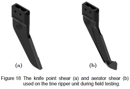
The objective of the first set of field tests, was to determine the effect of speed on the measured load components. Three different working speeds, 4 kmh^-1, 6 kmh^-1 and 8 kmh^-1, were chosen. The tests were conducted with both the knife point and aerator shears (figure 18) at the maximum working depth of each respective shear, while travelling in a straight line. The breakaway pressure was set at 11.5 MPa.

 

 

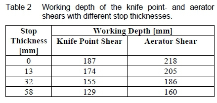
The second set of field tests was to determine the effect of different working depths on the measured load components. The working depth was set using specially designed stops with varying thicknesses, placed on the rods of the hydraulic cylinder controlling each wheel. For the first set of tests, no stops were inserted, and the implement was tested at the maximum working depth. For the subsequent tests, different thickness stops were used as shown in table 2. The tests were conducted at a speed of 6 kmh^-1 while travelling in a straight line. The breakaway pressure was set to 11.5 MPa.

 

 

The final set of field tests was to investigate the effect of the turning radius on the measured load components. Three different turning radii, 11.0 m, 15.5 m and 22.0 m were chosen. The radii were determined by locking the tractor's steering wheel at a fixed position and completing a full circle. The radius of the circle was then measured from the centre of the circle to the middle of the tracks left by the tractor's wheels. During this process, the measuring value (position) of the cable extension sensor was recorded. The mean value was then taken for each turning radius and used as a reference during the actual testing to maintain a constant turning radius.

 

7 Results and Discussion

The raw measurement data from the field tests were processed for each test configuration to determine the effect of speed, working depth, and turning radius, on the measured load components.

7.1 The Effect of Speed

Tests to determine the effect of speed (within the range of typical speeds used for planting/seeding) were completed with two different types of shears, namely the knife point and aerator shears, as shown in figure 18. The results shown, were obtained at a maximum working depth of 187 mm for the knife point shear, and 218 mm for the aerator shear. Both shears were tested while travelling in a straight line.

The effect of speed on the magnitude of the three orthogonal force components, as well as the resultant forces Rxy and Rxy_Z, is shown in figure 19. An increase of approximately 0.5 kN (11.9 %) in the mean draught force Fx is observed with an increase in speed from 4 kmh^-1 to 6 kmh^-1. From 6 kmh^-1 to 8 kmh^-1, the draught force stayed almost constant (increase of only 0.6 %). In all tests, the maximum draught force of 8.27 kN was observed for the knife point shear at a speed of 8 kmh^-1.

 

 

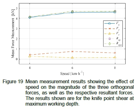
Like the draught force, the vertical force Fy also showed an increase of 0.32 kN (75.0 %) when the speed was increased from 4 kmh^-1 to 6 kmh^-1. The vertical force in turn decreased by 17.7 % when the speed was further increased from 6 kmh^-1 to 8 kmh^-1. Given the relatively low magnitude of the vertical force, an increase of 75.0 %, and decrease of 17.7 %, do not equate to much compared to the magnitude of the draught force and is therefore considered insignificant.

Both the Rxy and Rxyz resultant forces followed the same profile as the draught force with increasing speed. The close proximity of the resultant forces to the draught force, shows that the resultant forces were largely comprised of the draught force component. This further confirms the almost negligible effect of the observed vertical force fluctuations on the total force.

The lateral force Fz stayed relatively close to zero throughout the tests. This can be expected since the tests were performed in a straight line, with the shear having a thin width profile. The negligible effect of the lateral force is further confirmed by the small difference in the resultant forces Rxy and Rxyz for all the speed tests. A more prominent lateral force would have shown a clear difference between the two resultant forces.

Figure 20 shows the effect of speed on the mean moment for the knife point shear at maximum working depth. The results were consistent with the force data shown in figure 19, mainly since the profile of the main moment component Mz was consistent with that of the draught and resultant force components. The main moment increased by 13 % with a speed increase from 4 kmh^-1 to 6 kmh^-1, which is close to the 12 % increase observed in the draught force. The moment components Mx and My are shown to be negligible, which was expected since they were only influenced by the applied lateral force.

 

 

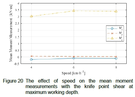
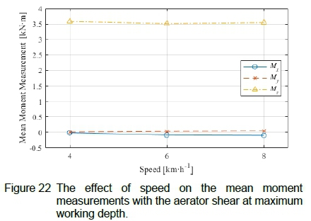
Figure 21 shows the effect of speed on the mean measurement of the three orthogonal force components and the respective resultant force components, using the aerator shear at maximum working depth. Unlike the tests with the knife point shear, the tests with the aerator shear showed no real difference in results with an increase in speed. This is also observed in the moment components as shown in figure 22.

 

 

 

 

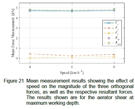
A slight difference in the mean measurements of the resultant force Rxyz is shown between the knife point shear and aerator shear. The mean resultant force Rxyz of the knife point shear over the three different speeds (nine tests in total), was 4.51 kN. The corresponding mean value for the aerator shear was 4.80 kN, 6.55 % higher than that of the knife point shear. Considering the variation in data (standard deviations reported below), this difference of 6.55 % is insignificant.

Given the results from the aerator shear, and since the difference in force with the knife point shear was only seen between 4 kmh^-1 and 6 kmh^-1, with no significant difference observed for higher speeds, it could be concluded that an increase in speed does not have a noticeable effect on the loads of both shears. These findings are consistent with [4] where a sweep type liquid manure injector was tested, with no speed effect observed.

The above conclusions were drawn based on the mean values. However, each test was repeated three times and the mean value and the standard deviation calculated for each. For the knife point shear, the standard deviation in the resultant force Rxyz (expressed as a percentage of the mean value) ranged from 5.9 % to 10.3 % over the range of speeds tested. For the aerator shear, the standard deviation ranged from 3.9 % to 5.4 %.

7.2 The Effect of Working Depth

The effect of working depth on the load components was investigated using the knife point shear at a travelling speed of 6 kmh¹.

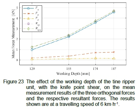
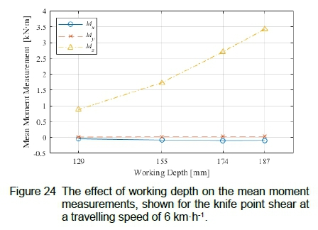
As expected, an increase in working depth resulted in an increase in the force components, figure 23. The same behaviour was observed for the main moment M_z, as shown in figure 24. The increase in the draught and vertical force components at deeper working depths, was consistent with the results of [4]. The mean resultant force Rxyz increased substantially (by 282.1%) from 1.23 kN at a working depth of 129 mm, to 4.68 kN at a maximum working depth of 187 mm. The increase appeared to be linear in nature (fitted straight lines with R² > 0.98), but since data of deeper working depth tests were not available, it would be premature to suggest that the increase would remain linear if the tine ripper unit were to be used at deeper working depths.

 

 

 

 

Since the tests were performed while travelling in a straight line, the lateral force Fz, together with the moment components M_xand My, were shown to be consistently near zero and were therefore negligible. The breakaway angle and vertical displacement of the ripper unit, as shown in figure 25, increased with an increase in working depth. As expected, a deeper working depth would result in more frequent breakaway to occur because of an increase in the resultant force Rxy. The noticeable increase in breakaway, from a working depth of 155 mm and higher, could be attributed to the composition of the soil. The soil comprised of a clay layer underneath a sandy loam crust. The clay layer was located relatively close to the surface. At a working depth of 155 mm, this clay layer was first encountered, from where the measured force and breakaway frequency increased as the working depth was increased.

 

 

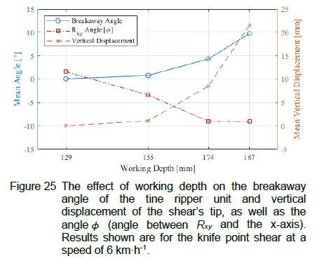
The angle φwas shown to increase in magnitude (with mostly negative values) with an increase in working depth. This is consistent with the increase in the vertical force component Fy shown in figure 23. As the shear penetrated deeper into the soil, the upward force exerted by the soil's clay layer on the shear also increased. A larger upward force component would in turn result in the angle between the resultant force Rxy and the horizontal to increase in magnitude (larger negative values). Since no real increase in the vertical force was seen between a working depth of 174 mm and 187 mm, the angle φalso remained constant.

For the knife point shear, the standard deviation in the resultant force Rxyz (expressed as a percentage of the mean value) ranged from 4.7 % to 10.6 % over the range of depths tested. For the aerator shear, the standard deviation ranged from 3.8 % to 8.3 %.

7.3 The Effect of Turning Radius

The effect of turning radii on the load components was investigated using the knife point shear at a speed of 6 kmh^-1 and at maximum working depth. Turning radii of 11.0 m, 15.5 m and 22.0 m were used for the tests. The results of the mean load components, as well as the respective resultant forces, are shown in figure 26.

 

 

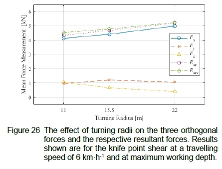
The lateral force component Fz decreased by 61.5 %, from 1.05 kN to 0.40 kN, as the turning radius increased from the minimum to the maximum value. This means that a larger lateral force was measured when the tractor and implement turned with a sharper (tighter) radius. This was expected since a sharper turn would result in the test setup to pivot on its inside rear wheel, inducing a lateral force on the tine. The resultant force measurements, together with draught force component, increased with an increase in turning radius. The increase in draught force could be attributed to the reduction in the lateral force component, resulting in a larger portion of the load being applied in the draught direction.

It was further observed that, as the lateral load decreased, the difference between the resultant forces Rxy and Rxyz, also decreased, indicating the effect of the lateral force on the resultant force Rxyz.

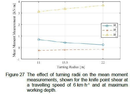
The results for the moment components are shown in figure 27. The large difference in perpendicular distance (782 mm and 69 mm measured from the shear's tip) between the lateral force component Fz and the x-axis and y-axis respectively, resulted in a smaller moment component My to be measured compared to the moment component Mx. The trend in the main moment component M_zwas similar to that of the resultant force Rxy.

 

 

 

8 Conclusion

A test setup, capable of measuring all the load components acting on tillage and planting implements, was successfully designed, manufactured, and tested. The setup consisted of a series of frames, sliding relative to each other on sets of linear bearings, and load cells to measure the force and moment components. The main frame formed a trailer, simulating the same operational conditions as experienced by implements drawn behind a tractor.

The laboratory-controlled testing, as well as the field tests, showed that the setup could be used to accurately determine the three orthogonal force components and their respective moments. The ability to isolate and accurately measure each of the three orthogonal load components, while showing minimal cross-interference with the other measuring directions, was demonstrated. The main moment component Mz, comprising of the draught and vertical load components Fx and Fy, could also be accurately measured. The remaining moment components Mx and My could then be calculated using the measured force and geometric position data. Finally, the direct frequency, induced on the implement by the soil, was measured by a set of strain gauges installed on the implement, close to the point of contact with the soil. This data was used to apply a low-pass filter to the load cell data to eliminate unwanted higher frequencies.

Data obtained with the test setup will be valuable in the future design of implements. It can be used to perform accurate design calculations, used as input to FEM simulations, and to perform accurate fatigue analyses. The implement designs can therefore be improved to better withstand their specific operational conditions. This would also increase the useable lifespan of the implements, justifying the large capital expenditure by farmers to acquire these implements.

 

Acknowledgements

Equalizer AG (Pty) Ltd supported this project by supplying equipment and materials. J. W. van Santen was financially supported by the National Research Foundation.

 

References

[1] M. T. Knudsen, N. Halberg, J. E. Olesen, J. Byrne, V. Iyer, and N. Toly. Global trends in agriculture and food systems. Global development of organic agriculture-challenges and prospects, Cabi Publishing, pp 1-48, 2006.

[2] Trends in the Agricultural Sector 2017, Department of Agriculture, Forestry and Fisheries, South Africa, URL: https://www.dalrrd.gov.za/Resource-Centre?folderId=377, 2018.

[3] J. Khan, R. J. Godwin, J. Kilgour and B. S. Blackmore. Design and calibration of a bi-axial extended octagonal ring transducer system for measurement of tractor-implement forces. Journal of Engineering and Applied Sciences, 2(1):16-20, 2007.         [ Links ]

[4] Y. Chen, N. B. McLaughlin and S. Tessier. Double extended octagonal ring (DEOR) drawbar dynamometer. Soil and Tillage Research, 93(2):462-471, 2007.         [ Links ]

[5] L. L. Kasisira and H. L. M. Du Plessis. Energy optimization for subsoilers in tandem in sandy clay loam soil. Soil and Tillage Research, 86(2):185-198, 2006.         [ Links ]

[6] J. Pijuan, J. Berga, M. Comellas, X. Potau and J. Roca. A three-point hitch dynamometer for load measurements between tillage implements and agricultural tractors during operation. URL: https://www.researchgate.net/publication/267405934

[7] H. Bentaher, E. Hamza, G. Kantchev, A. Maalej and W. Arnold. Three-point hitch-mechanism instrumentation for tillage power. Biosystems Engineering, 100(1):24-30, 2008.         [ Links ]

[8] N. Nobakht, M. Askari, A. M. Nikbakht and Z. Ghorbani. Development of a dynamometer to measure all forces and moments applied to tillage tools. MAPAN, 32(4):311-319, 2017.         [ Links ]

[9] C. J. Coetzee and D. N. J. Els. Calibration of granular material parameters for DEM modelling and numerical verification by blade-granular material interaction. Journal of Terramechanics, 46(1):15-26, 2009.         [ Links ]

[10] MecVel. Linear actuator EC5 AC, URL: https://www.mecvel.com/linear-actuator-ec05-ac/.

[11] M. Popov. The influence of vibration on friction: A contact-mechanical perspective. Frontiers in Mechanical Engineering, 6(69), 2020.         [ Links ]

[12] QuantumX MX840B/MX440B: Universal Data Acquisition Module | HBM. URL: https://www.hbm.com/en/2129/quantumx-mx840b-8-channel-universal-amplifier/.

 

 

Received 5 October 2021
Revised form 17 December 2021
Accepted 9 May 2021