Pressure Recovery Discharge Configurations for an Induced Draught Axial Flow Fan

 

 

G. M. Bekker^I; C. J. Meyer^II; S. J. van der Spuy^III

^IDepartment of Mechanical and Mechatronic Engineering, Stellenbosch University, South Africa. E-mail: 17732956@sun.ac.za
^IIAssociate Professor. Department of Mechanical and Mechatronic Engineering, Stellenbosch University, South Africa. E-mail: cjmeyer@sun.ac.za
^IIISAIMechE Member, Professor. Department of Mechanical and Mechatronic Engineering, Stellenbosch University, South Africa. E-mail: sjvdspuy@sun.ac.za

 

 

---

ABSTRACT

This study investigates the potential gains in operating volume flow rate and static efficiency of an induced draught axial flow fan system. These gains are achieved through pressure recovery, i.e. the conversion of dynamic pressure at the fan exit into static pressure. Pressure recovery is achieved using downstream diffusers, stator blade rows, and combinations of these. Three different diffuser lengths are considered. Of the shortest diffusers, a conical diffuser increases the operating volume flow rate by 3.2 % and the fan static efficiency by 9.8 % (absolute). A longer conical diffuser increases it by 3.9 % and 11.9 %, respectively. Of the longest diffusers, an annular diffuser increases the flow rate by 5.5 % and the fan static efficiency by 16.8 %.

Additional keywords: Pressure recovery, axial flow fan, induced draught, diffuser, stator.

---

 

 

Nomenclature Roman

A Area [m²]

AR Diffuser area ratio

a Curve fitting coefficient [kg/m⁷]

C_DDrag coefficient

C_LLift coefficient

d Diameter [m]

F Force [N]

K_difDiffuser total pressure loss coefficient

K_recPressure recovery coefficient

𝐾_*rec Pressure recovery coefficient as per Bekker et al. [1]

k Turbulence kinetic energy [m²/s²]

I Length [m]

P_FFan power consumption [W]

ρ Pressure [Pa]

r Radius [m]

t Actuator disc thickness [m]

V, V Volume [m³]; and volume flow rate [m³/s]

νVelocity [m/s]

y Wall-normal distance [m]

y⁺ Sublayer-scaled wall-normal distance

Greek

𝛼_eKinetic energy flux correction factor

βRelative flow angle [deg]

β₁ Turbulence model constant, 0.075

Δ, δ Difference; and small difference

ηEfficiency [%]

θDiffuser half-wall angle [deg]

νKinematic molecular viscosity [m²/s]

ρDensity [kg/m³]

σBlade solidity

ω Turbulence specific dissipation rate [s^-1]

Subscripts

des Design point

dif Diffuser

down Downstream

dump Dump representing the open atmosphere

e Exit (fan or diffuser outlet)

F Fan

FC Fan casing

F/dif Fan-diffuser unit

F/difs Fan-diffuser static

FH Fan hub

Fs Fan static

Ft Fan total

HE Heat exchanger

i Inlet or inner diffuser wall

inlet Inlet boundary

max Maximum

0 Outlet or outer diffuser wall op Operating point

R Relative

s Static

t Total (or stagnation)

up Upstream

𝑥,𝜃Axial and tangential directions

∞Atmospheric conditions

Abbreviations

ACC Air-cooled condenser

ADM Actuator disc model

CFD Computational fluid dynamics

DILU Diagonal-based incomplete LU preconditioner

EADM Extended actuator disc model

GAMG Geometric-algebraic multi-grid solver

PBiCG Preconditioned bi-conjugate gradient solver

SIMPLE Semi-implicit method for pressure-linked equations

 

1 Introduction

This research focuses on improving the performance of an axial flow fan to be used in an induced draught air-cooled condenser (ACC). Such ACCs employ large arrays of axial flow fans to draw air through heat exchanger bundles in order to condense the process fluid inside the heat exchanger tubes.

The improvement in fan performance was achieved through pressure recovery. Pressure recovery refers to the conversion of dynamic pressure at the fan outlet into static pressure. The effect of pressure recovery is to increase the effective fan static pressure rise. In an ACC fan unit, the fan curve and resistance curve then intersect at a higher fan static pressure and airflow rate. The increased airflow rate through the heat exchangers allows for higher heat rejection rates from the process fluid to the air. The increased fan static pressures also translate to improved operating fan static efficiencies.

Bekker et al. [1] reported significant gains in fan performance due to pressure recovery. They examined six different types of discharge configurations for an axial flow fan: For the first type, the fan was followed by a stator blade row. Conical diffusers comprised the second type. The third type combined the stator and conical diffusers so that the stator followed the fan and the diffusers followed the stator blade row. The fourth and fifth types involved annular diffusers with and without a stator blade row between the fan and diffusers. The sixth and final outlet configuration had a stator blade row fitted at the outlet of an annular diffuser.

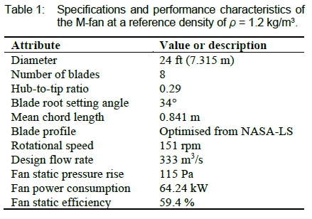
Bekker et al. [1] used the M-fan for their study. This fan was designed by Wilkinson et al. [2] to be used in modern ACCs. Table 1 summarises the attributes of the M-fan along with its performance characteristics at its design flow rate.

 

 

The current study expands on the work of Bekker et al. [1]. The same discharge configurations are considered for the same axial flow fan. The theory and modelling strategies outlined in Bekker et al. [1] also apply here. However, Bekker et al. [1] investigated only a single diffuser length equal to the fan diameter, i.e. 7.315 m. They also used conservative axial clearances between the fan, stator rows, and diffusers. The overall length of the discharge configurations considered by Bekker et al. [1] ranged between 9.24 and 10.53 metres. Such lengths, however, are considered impractical.

Furthermore, as per BS EN ISO 5801 [3], Bekker et al. [1] assumed the static pressure at the fan outlet to be equal to atmospheric pressure. However, Bekker et al. [4] established that the static pressure at the fan outlet is, in fact, lower than atmospheric pressure. The result is that the pressure recovery coefficients presented in Bekker et al. [1] are optimistic.

Consequently, shorter discharge diffusers were investigated in the current study. Less conservative axial clearances between turbomachinery blading and diffusers were also used. Additionally, pressure recovery coefficients were calculated using the more conservative formula suggested by Bekker et al. [4].

Two shorter diffuser lengths equal to 40 % and 20 % of the fan diameter were considered. That is, 2.926 and 1.463 metres, respectively. Kröger [5] portrays a diffuser of a length equal to /_dif= 0.4cZ_F (where d_Fis the fan diameter) as a "practical diffuser".

At the start of the paper, pressure recovery theory is revised to illustrate how pressure recovery influences axial flow fan performance in induced draught systems. Detail pertaining to the numerical simulation approach follows. Pressure recovery coefficients obtained with different discharge configurations for the M-fan are presented next. These were obtained at the design flow rate of the fan. The configurations producing the highest pressure recoveries at the design flow rate were investigated further at off-design flow rates. Finally, the pressure recovery data of the most promising discharge configurations of each length were added to the performance characteristics of the M-fan. This allows for comparison between the fan-diffuser and M-fan characteristics. A summary of the main findings concludes the paper.

 

2 Pressure Recovery Theory

Figure 1 depicts a fan system representative of an induced draught ACC. The draught equation for this system is given by (see the appendix for a detailed derivation)

 

 

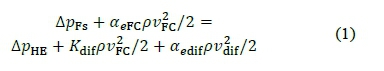
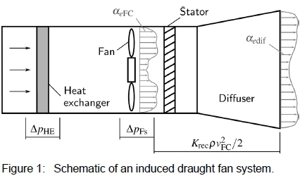
On the left-hand side of equation (1), energy is supplied to the system by the axial flow fan. From left to right, Ap_Fs is the fan static pressure rise, a_eFC is the kinetic energy flux factor at the fan exit, ρis the air density, and v_FC = V/A_FCis the mean axial velocity through the fan casing. The terms on the right-hand side of equation (1) represent the energy dissipated as air passes through the system. From the left again, Δp_HE represents the static pressure loss due to the heat exchanger and K_difis the total pressure loss coefficient of the diffuser. At the outlet of the diffuser, a_ediíis the kinetic energy flux factor and v_dii = 𝑉/A_difis the mean axial velocity.

According to Kröger [5], a_eFC, K_diiand a_ediiare normally unknown and troublesome to measure. Therefore, Bekker et al. [1] moved these terms to the left-hand side of equation (1) and grouped them to form a pressure recovery coefficient. This coefficient is obtained by normalising this group of terms with the mean axial dynamic pressure through the fan casing so that

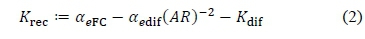
where AR = A_dif/A_FC is the area ratio of the diffuser.

Substituting equation (2) into equation (1) simplifies the draught equation to

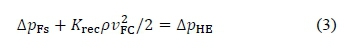
If Krec = ^ae_FC, the effective fan pressure rise would equal the fan total pressure rise, i.e. 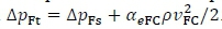This would result in the highest operating flow rate theoretically possible, V_max. However, continuity requires that a_edif > 1 and diffuser stall limits AR. Furthermore, viscous and local losses in the diffuser translate to 𝛼_dif > 0.

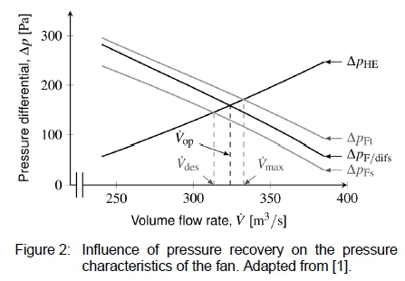
The static pressure characteristics of the fan-diffuser unit, 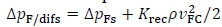, will therefore be higher than the static pressure characteristics of the fan but lower than the fan's total pressure characteristics (see figure 2). Figure 2 further illustrates how pressure recovery shifts the operating point of the fan system to a higher operating volume flow rate, V_op, compared to the initial design flow rate, 7_des.

 

 

Induced draught ACCs fitted with appropriate discharge configurations could therefore operate at flow rates that are higher than the design flow rate. Owing to the increased mass flow rate of air though the heat exchangers, the ACC will be capable of transferring more heat from the process fluid to the atmosphere.

 

3 Numerical Approach

Because of the large physical size of ACC fans, full-scale testing is considered impractical. Furthermore, the number of discharge configurations that had to be tested was significant. By means of computational fluid dynamics (CFD), it was possible to obtain pressure recovery data for a total of 548 outlet configurations for the M-fan. Computations were performed employing the open-source CFD code, OpenFOAM 5.0.

3.1 Numerical validation

Prior to the simulation of the different discharge configurations, the CFD approach was validated against the experimental data of Clausen et al. [6] for swirling flow in a conical diffuser. Full details of the validation study are available in Bekker et al. [1].

Bekker et al. [1] tested various high- and low-Reynolds-number turbulence models and found that the wall-integrated k-ωmodel of Wilcox [7] produced reasonable results. Since it was found that results were sensitive to the specified inlet turbulence quantities, it was decided to use profiles for turbulence quantities that Wilkinson [8] measured downstream of the M-fan. Furthermore, Bekker et al. [1] found that steady-state simulations performed on two-dimensional axisymmetric meshes produced results on par with transient and three-dimensional simulations.

3.2 Computational domain and mesh

The computational domain for one of the more complex discharge configurations for the M-fan is depicted in figure 3a. It is the domain that was used for the annular diffusers fitted with a stator row at their inlets.

 

 

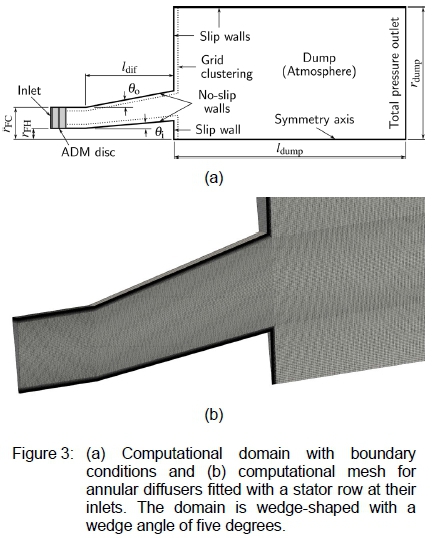
Block-structured meshes comprising of hexahedral cells were generated using Open FOAM's blockMesh utility (see figure 3b). The meshes were wedge-shaped, consisting of a single computational cell in the tangential direction. The wedge angle was set to five degrees, as recommended by Greenshields [9] for axisymmetric flow problems. Grid-clustering at solid surfaces facilitated integration through the boundary layer. The width of such a clustered zone was 5 % of the fan diameter and had a high degree of grading towards the wall. The grading allowed for y⁺~1 at the walls and a smooth transition with the inner mesh.

3.3 Boundary conditions

The inlet of the domain was located at one-half mean fan-blade chord length downstream of the M-fan. The fan itself was thus not modelled. Instead, fixed velocity and turbulence profiles at the fan outlet were used to specify the inlet boundary conditions. These profiles were obtained from Wilkinson [8] for flow rates ranging from 260 to 380 m³/s. These profiles were computed using a three-dimensional periodic fan model with no tip clearance.

It is reasonable to assume that downstream stator blade rows or diffusers will not significantly alter the flow profiles exiting the fan: Terzis et al. [10] found that outlet guide vanes did not alter the velocity profiles at the outlet of a small fan. And Bekker et al. [4] obtained similar velocity profiles at the outlet of the M-fan with or without discharge diffusers. Along with the velocity and turbulence profiles specified at the inlet, a zero-gradient condition was assigned to pressure.

The remainder of the boundary conditions are displayed in figure 3: At no-slip surfaces, k = 0, ω = 6v/(ß_iy²) [11], and Vp = 0 were used. A fixed total pressure of zero was assigned to the outlet boundary along with zero gradients for velocity and turbulence quantities. In the case of reverse flow at the outlet, velocity was calculated from the flux in the boundary-normal direction. Wedge boundaries were specified for the axisymmetric planes. These function as cyclic boundaries for two-dimensional axisymmetric problems in OpenFOAM. A symmetry condition was applied to the axisymmetric axis of the domain.

3.4 Numerical solver settings

Simulations devoid of stator blade rows employed a steady-state solver for incompressible flows with turbulence, i.e. the simpleFoam solver. When stator blade rows required modelling, the extended actuator disc model (EADM) of Van der Spuy [12] was used. Engelbrecht [13] incorporated this model into the buoyantBoussinesqSimpleFoam solver of OpenFOAM. Both mentioned solvers employ the SIMPLE algorithm to solve the continuity and momentum equations. The following section provides more detail regarding the EADM.

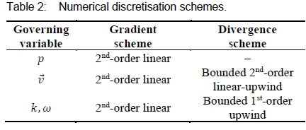
Table 2 provides the discretisation schemes that were used for the gradient and divergence terms. The discretisation of Laplacian terms requires an interpolation scheme and a surface-normal gradient scheme. The former was achieved using linear interpolation from cell centres to face centres. The surface-normal gradients were discretised using a limited-corrected scheme with a relaxing coefficient of 0.33.

 

 

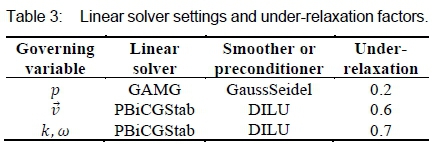
The linear solvers that were used for each governing variable are listed in table 3. This table also contains the under-relaxation factors that were used for the iterative solution procedure.

 

 

The kinematic viscosity and density of air at 20 °C were used, i.e. kg/m³, respectively. Solutions were deemed converged after the static pressure at the domain inlet settled to a constant value and the scaled residuals reduced to 10^-4 or lower.

3.5 Sensitivity studies

The computational mesh density was increased up to a point where the computed pressure recovery coefficient changed by less than two per cent compared to the result obtained with the previous coarser mesh. In addition, the velocity profiles at the outlet of the discharge configurations using successively refined meshes had to be near identical before considered grid-independent.

For each type of fan-outlet configuration, the sensitivity to the size of the discharge dump that represented the open atmosphere was investigated (see figure 3). The dump size (r_dump and 𝑙 _dump) was increased up to a point where the pressure recovery and velocity profiles no longer changed.

 

4 Stator Modelling

Stator blade rows were modelled using the extended actuator disc model (EADM) of Van der Spuy [12]. This model employs isolated aerofoil data to compute the force a fan blade would exert on air. The force is introduced into the momentum equation through a source term. The axial component of the source term is calculated as

and the tangential component as

In the above equations, v_Rand βare the relative velocity vector and flow angle, σis the blade solidity, and t is the thickness of the actuator disc. The lift and drag coefficients, C_Land C_D, are obtained from isolated aerofoil data.

In order to compute the source terms described by equations (4) and (5), the model requires the blade chord and stagger angle distributions. These distributions were computed using the isolated aerofoil design method outlined in Louw et al. [14].

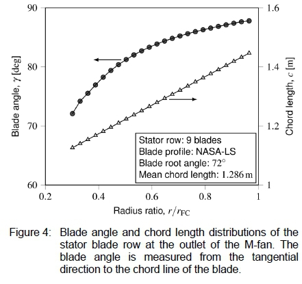
A nine-bladed stator row with the blade angle and chord length distributions in figure 4 was capable of removing all the swirl exiting the M-fan at the design flow rate. As recommended by Wallis [15], the stator was located at a half mean rotor chord length downstream of the fan.

 

 

For the discharge configurations where stator blade rows were installed at the outlet of annular diffusers, new stator rows had to be designed. In order to obtain realistic chord lengths, these stator rows required 13 blades and could remove only ~50 % of the swirl exiting the annular diffusers.

 

5 M-fan Discharge Configurations

Similar to Bekker et al. [1], various discharge configurations were investigated for the M-fan. The aim was to find configurations producing high pressure recovery coefficients at both design and off-design conditions. After identifying the most promising discharge configurations, their pressure recovery data were added to the characteristics of the M-fan. The characteristics of the M-fan and fan-diffuser units could then be compared to quantify the gains in performance due to pressure recovery.

5.1 Calculation of pressure recovery

Bekker et al. [1] computed the pressure recovery coefficient of a discharge configuration as

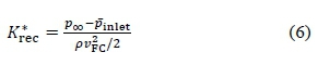
where is the area-weighted static pressure measured at the inlet of the computational domain and is equal to atmospheric pressure. BS EN ISO 5801 [3] stipulates that the static pressure at the fan outlet in equation (6) should be assumed to be equal to atmospheric pressure. In other words, without any discharge configuration recovering pressure, should be true so that

Bekker et al. [4], however, established that p_inlet < p_o even though no downstream stator blade row or diffuser was present. For the fan on its own, equation (6) thus erroneously yields if_r*_ec > 0. Bekker et al. [4] therefore analysed the fan exit region without any discharge configuration. The same velocity and turbulence profiles of Wilkinson [8] were utilised to obtain the average static pressure at the fan outlet at different flow rates. They then corrected equation (6) as follows:

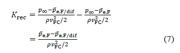
where p_eF is the area-weighted static pressure measured at the domain inlet (which corresponds to the fan outlet) without any discharge configuration and is measured in the same manner but with a discharge configuration. Bekker et al. [4] demonstrated that equation (7) is more conservative than equation (6), especially at lower off-design flow rates. The pressure recovery coefficients presented in the sections to follow were computed using equation (7).

5.2 Pressure recovery at design conditions

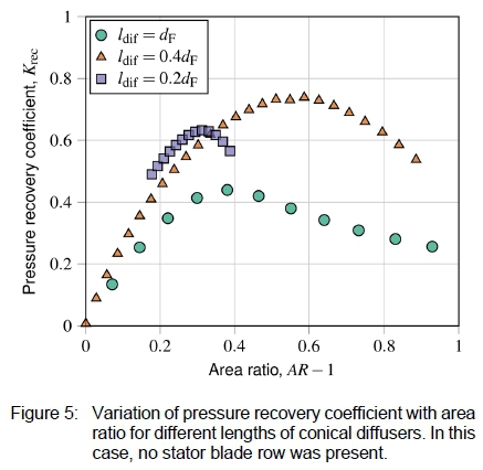
Parametric studies were performed at the fan's design flow rate of 333 m³/s. For each diffuser length, the area ratio was varied by changing the divergence angle of the diffuser.

For the conical diffusers of length Z_dif = d_F, the half-wall angle (angle between the axial direction and diffuser wall) was varied within the range of 0° < 0 < 20° in increments of one degree. Half-wall angles of 0° < 0 < 25° were tested for conical diffusers of length Z_dif = 0.4cZ_F. And the shortest diffusers, /_dif = 0.2cZ_F, were tested in a narrower range of 8° < 0 < 24°.

Figure 5 depicts the pressure recovery data for the different area ratios that were tested. These results were obtained with no stator blade row present. The same procedure was followed for the conical diffusers with a stator row located between the fan outlet and diffuser inlet.

 

 

For the configurations involving annular diffusers, numerous combinations of inner and outer half-wall angles were tested. The inner half-wall angle was varied within the range of 0° < 0¡ < 30° in increments of two degrees for the longest diffusers, i.e. ζ_dif = cZ_F. A range of outer half-wall angles, 0_o, was tested for each of these inner half-wall angles. The ζ _dif = 0.4d_F diffusers were tested for -10° < 0¡ < 30° in increments of two degrees. Finally, the ζ_dif = 0.2cZ_F diffusers were tested in larger increments of four degrees in the range of -20° < 0¡ < 8°.

Evidently, considerably more simulations were required to obtain the annular diffuser geometry producing the highest pressure recovery coefficient for each diffuser length compared to the conical diffuser cases. That is, similar to figure 5, a pressure recovery coefficient versus area ratio graph could be constructed for each inner half-wall angle that was investigated.

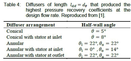
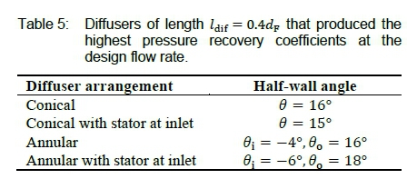
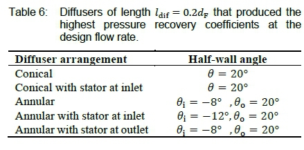
Following the above procedure, it was possible to identify the most promising diffuser geometries for each type of discharge configuration. The geometries of the best performing diffusers for the M-fan at the design flow rate are summarised in tables 4 to 6.

5.3 Pressure recovery under off-design conditions

The fans in ACCs often operate under off-design conditions: Louw et al. [16] found that the fans along the periphery of an induced draught ACC operate at slightly reduced flow rates due to flow separation along the sides of the ACC. They also reported that wind significantly reduces fan performance, especially in the wind-facing periphery units. Additionally, fouling could alter the operating point of a fan unit [5]. It is therefore important to determine how the different discharge configurations perform under off-design conditions.

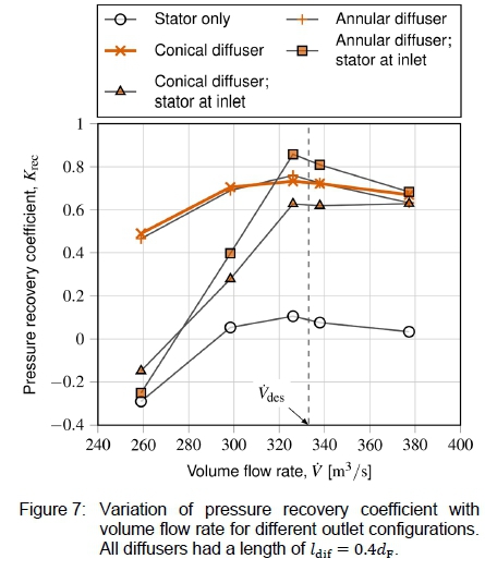
The discharge configurations listed in tables 4 to 6 were evaluated at flow rates ranging from 260 to 380 m³/s. The pressure recovery coefficients obtained at these flow rates are presented in figures 6 to 8.

 

 

 

 

 

 

 

 

 

 

 

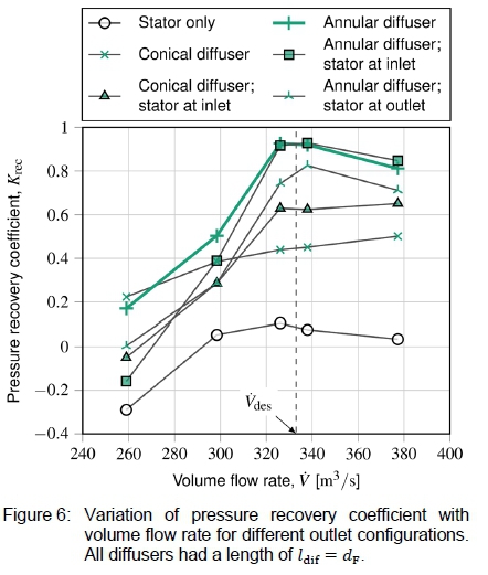
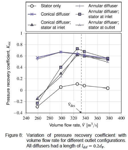
In every instance where a stator blade row is combined with a diffuser, the pressure recovery coefficient deteriorates significantly at lower off-design flow rates. The stator row on its own, however, does not exhibit such a large sensitivity to the flow rate. This suggests that the diffusers in the statordiffuser combinations are responsible for the decline in pressure recovery at off-design flow rates.

With the stator row located between the fan outlet and diffuser inlet, the velocity profiles exiting the stator row at off-design flow rates are no longer conducive for diffuser performance. With stator rows at the annular diffuser outlets, the velocity profiles entering the stators are different from what the stators were designed for, as they were designed for the design flow rate. This results in increased losses in the stator row, which reduces pressure recovery. The discharge configurations featuring stator blade rows are therefore considered unsuccessful.

Comparing the conical and annular diffuser results in figure 6 (without stator rows), the annular diffuser produces considerably higher pressure recovery coefficients. The annular diffuser with equiangular walls of 22° is therefore recommend for the l_dif = d_Fcase.

The conical and annular diffusers for the shorter diffuser lengths yield essentially identical pressure recovery coefficients (see figures 7 and 8). Since conical diffusers require less material to manufacture and are simpler to install, they are recommended for the /_dif= 0.2 d_Fand /_dif= 0.4cZ_F lengths.

5.4 Effect of pressure recovery on fan performance characteristics

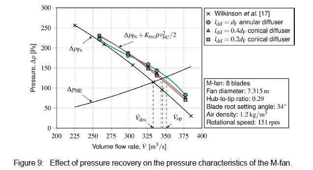
The pressure recovery data of the diffusers recommended in the previous section were added to the characteristics of the M-fan to obtain the combined fan-diffuser characteristics. For the /_dif= d_Flength, the 22° equiangular annular diffuser was recommended. For the /_dif= 0.4 d_F length, it was the conical diffuser with an included angle of 2θ= 32°. For the ζ_dif= 0.2d_F length, the 2θ = 40° conical diffuser was recommended.

Figure 9 depicts the static pressure characteristics. The fan characteristics were obtained from Wilkinson et al. [17], who used a periodic three-dimensional fan model with no tip clearance. A system curve representing the pressure drop of a typical heat exchanger was included in figure 9. It served to estimate the new operating points of the fan system after adding the diffusers. The pressure drop takes the general form of . The curve passes through the origin and the design point of 115 Pa at 333 m³/s.

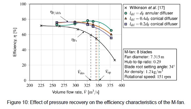
The static efficiency characteristics of the fan and fandiffuser combinations are displayed in figure 10. The static efficiency of the fan was calculated as

where P_Fis the shaft power supplied to the fan. For the fandiffuser combinations, the efficiency was calculated with

where . Note that in both equations (8) and (9), the same fan power characteristics were used. Hence, it is assumed that the added diffusers do not alter the power characteristics. This is a reasonable assumption, as Bekker et al. [4] simulated scaled versions of these exact fan-diffuser combinations and found that the diffusers had no marked impact on the power characteristics.

The pressure recovery of the annular diffuser of length ζ_dtf = d_Fincreased the flow rate through the fan from 333 to 351 m³/s. Thus, a relative increase of 5.5 %. The fan static efficiency rose from 59.4 % at the initial design point to 76.2 % at the new operating point. Thus, an absolute increase of 16.8 %.

The ζ_dif= 0.4d_F conical diffuser shifted the operating flow rate to 346 m³/s, which is a 3.9 % increase. The resulting operating fan static efficiency was 71.3 %, which is 11.9 % (absolute) higher than without the diffuser.

Finally, the ζ_dif= 0.2d_F conical diffuser shifted the operating point to 123 Pa at 344 m³/s, yielding a fan static efficiency of 69.2 %. The flow rate and static efficiency thus rose by 3.2 % (relative) and 9.8 % (absolute), respectively.

 

6 Conclusions

This research followed on the work of Bekker et al. [1]. However, more practical (shorter) exhaust diffusers were also considered. Furthermore, pressure recovery coefficients were computed using the more conservative formula suggested by Bekker et al. [4].

The theory of pressure recovery for an axial flow fan in an induced draught system was revised. Pressure recovery data for various discharge configurations added to the M-fan were also provided. These configurations included combinations of conical and annular diffusers fitted with or without stator blade rows at their inlets. Cases with stator blade rows at the outlets of annular diffusers were also investigated. Three different diffuser lengths were considered for each type of discharge configuration.

The longest diffusers had a length equal to the fan diameter of 7.315 m. In this case, an annular diffuser with equiangular walls at 22° from the axial direction produced the highest pressure recovery coefficients over the considered range of flow rates. This diffuser increased the volume flow rate through the M-fan by 5.5 % relative to the initial design flow rate of 333 m³/s. The fan static efficiency also rose from 59.4 % to 76.2 %, i.e. an absolute increase of 16.8 %.

The mid-length diffusers had a length equal to 40 % of the fan diameter (i.e. 2.926 m). In this case, a conical diffuserwith a divergence angle of 20 = 32° performed well over the considered range of flow rates. With this diffuser, the volume flow rate through the fan was 3.9 % higher than the initial design flow rate and the fan static efficiency was 11.9 % (absolute) higher at the new operating point.

The shortest diffusers were 1.463 m long, or 20 % of the length of the fan diameter. Of these configurations, a conical diffuser with a divergence angle of 20 = 40° produced the most promising pressure recovery coefficients over the considered range of flow rates. The flow rate through the fan increased by 3.2 % relative to the initial design flow rate due to the added diffuser. The fan static efficiency rose by 9.8 %.

 

References

[1] G. M. Bekker, C. J. Meyer and S. J. Van der Spuy. Numerical investigation of pressure recovery in an induced draught fan arrangement. R & D Journal. 36:1928, 2020.         [ Links ]

[2] M. B. Wilkinson, S. J. Van der Spuy and T. W. Von Backström. The Design of a Large Diameter Axial Flow Fan for Air-Cooled Heat Exchanger Applications. InASME Turbo Expo 2017: Turbomachinery Technical Conference and Exposition, Charlotte, NC, USA, 2017.

[3] BS EN ISO 5801. Industrial fans - Performance testing using standardized airways. British Standard Institution, 2008.

[4] G. M. Bekker, C. J. Meyer and S. J. Van der Spuy. Performance enhancement of an induced draught axial flow fan through pressure recovery. R & D Journal. 37:35-44, 2021.         [ Links ]

[5] D. G. Kröger. Air-cooled heat exchangers and cooling towers: Thermal-flow performance evaluation and design. Department of Mechanical Engineering, Matieland, 1998.

[6] P. D. Clausen, S. G. Koh and D. H. Wood. Measurements of a swirling turbulent boundary layer developing in a conical diffuser. Experimental Thermal and Fluid Science. 6(1):39-48, 1993.         [ Links ]

[7] D. C. Wilcox. Turbulence Modeling for CFD. 2^nd ed. DCW Industries, 1998.

[8] M. B. Wilkinson. The design of an axial flow fan for air-cooled heat exchanger applications. Master's Thesis, Department of Mechanical and Mechatronic Engineering, Stellenbosch University, 2017.         [ Links ]

[9] C. J. Greenshields. OpenFOAM: User Guide. 5^th ed. OpenFOAM Foundation Ltd., 2017.

[10] A. Terzis, I. Stylianou, A. I. Kalfas and P. Ott. Heat transfer and performance characteristics of axial cooling fans with downstream guide vanes. Journal of Thermal Science. 21(2):162-171, 2012.         [ Links ]

[11] D. C. Wilcox. Reassessment of the scale-determining equation for advanced turbulence models. AIAA Journal. 26(11):1299-1310, 1988.         [ Links ]

[12] S. J. Van der Spuy. Perimeter fan performance in forced draught air-cooled steam condensers. PhD Thesis, Department of Mechanical and Mechatronic Engineering, Stellenbosch University, 2011.         [ Links ]

[13] R. A. Engelbrecht. Numerical investigation of fan performance in a forced draft air-cooled condenser. PhD Thesis, Department of Mechanical and Mechatronic Engineering, Stellenbosch University, 2018.         [ Links ]

[14] F. G. Louw, P. R. P. Bruneau, T. W. Von Backström and S. J. Van der Spuy. The design of an axial flow fan for application in large air-cooled heat exchangers. In ASME Turbo Expo 2012: Turbomachinery Technical Conference and Exposition, Copenhagen, Denmark, 2012.

[15] R. A. Wallis. Axial flow fans and ducts. John Wiley & Sons, 1983.

[16] D. L. Louw, C. J. Meyer and S. J. Van der Spuy. Numerical investigation of an induced draft air-cooled condenser under crosswind conditions. In ASME 2021 Summer Heat Transfer Conference, June 16-18, Virtual conference, Online, 2021.

[17] M. B. Wilkinson, S. J. Van der Spuy and T. W. Von Backström. Performance Testing of an Axial Flow Fan Designed for Air-Cooled Heat Exchanger Applications. In ASME Turbo Expo 2018: Turbomachinery Technical Conference and Exposition, Oslo, Norway, 2018.

 

 

Received 21 September 2021
Revised form 27 December 2021
Accepted 17 January 2022

 

 

Appendix

The draught equation for the system in figure 1 is obtained by subtracting the total pressure far downstream of the system from the total pressure far upstream of the system, i.e.

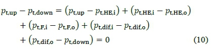
where are assumed. In equation (10) and the equations to follow, subscripts "t" and "s" denote total and static pressures, respectively. Subscripts "i" and "o" refer to the inlet and outlet sides of components, respectively. Furthermore, "F", "HE" and "dif" subscripts denote fan, heat exchanger and diffuser, respectively.

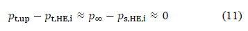
The dynamic pressure at the inlet of the system is deemed negligible so that

Assuming that the dynamic pressures at the inlet and outlet of the heat exchanger are equal, the total pressure difference across the heat exchanger simplifies to

In BS ISO 5801 [3], the fan total pressure is defined as 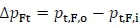and the fan static pressure is defined as 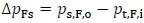. The total pressure difference across the fan can therefore be expressed as

where is the dynamic pressure at the fan outlet.

The total pressure loss across the diffuser-stator discharge configuration is given by

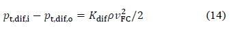
Finally, as per BS ISO 5801 [3], the dynamic pressure at the system outlet is assumed to be lost so that

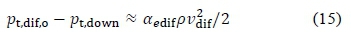
which implies that

Substituting equations (11) to (15) into equation (10) and rearranging yields the draught equation that was given in equation (1).