ARTICLES

 

Simulating Turbulent Air Flow Past a Hemispherical Body

 

 

M.R. Meas^I; J.F. Bruwer^II; M.L. Combrinck^III; T.M. Harms^II

^IDepartment of Mechanical and Mechatronic Engineering, Stellenbosch University, South Africa. E-mail: mmeas@sun.ac.za (corresponding author)
^IIDepartment of Mechanical and Mechatronic Engineering, Stellenbosch University, South Africa
^IIIDepartment of Mechanical and Construction Engineering, Northumbria University, Newcastle, United Kingdom

 

 

---

ABSTRACT

The flow of air past a smooth surface-mounted hemisphere is investigated numerically using six common RANS turbulence models and seeking steady flow solutions. Where possible, the turbulence models are applied using standard wall functions, resolving the viscous sublayer, and the enhanced wall treatment option in ANSYS Fluent. Results of the simulations are compared against measurements taken in a wind tunnel experiment. The comparison shows that enhanced wall treatment and resolving the boundary layer on a low Reynolds number mesh yields superior accuracy compared to standard wall functions or resolving the boundary layer on a high Reynolds number mesh, for all the turbulence models considered. The RNG k - ε model with enhanced wall treatment applied is found to yield the most accurate prediction of the static pressure distribution across the surface of the hemisphere model. Conversely, the Reynolds Stress model and the standard k - ω model are found to give the least accurate predictions, irrespective of the near-wall modelling approach applied. It is found that good agreement with the experimental data for this case offlows can be attained using each of the near-wall modelling techniques if a well-suited turbulence model is used.

Keywords: hemisphere, wind tunnel, turbulence modelling, computational fluid dynamics, steady flow

---

 

 

Nomenclature Roman

C_ppressure coefficient,

p pressure [Pa]

Re Reynolds number

mean free stream velocity in X direction [m/s]

Greek

α angular position along the centreline [°]

ρ density of fluid [kg/m³]

Subscripts

0 free stream

 

1 Introduction

Curved structures are prevalent throughout the natural and built environment in the form of domed buildings, fixtures on aircraft and marine vessels, and some species of plants. Understanding of the flow regimes near highly curved bodies is of interest in many fields of study and may be prompted by the need to assess wind or heat loads on domed structures, or deposition of substances such as pollutants, snow, or seeds in the vicinity of such objects.

Existing literature shows that the flow field established around the relatively simplistic geometry of a hemisphere is indeed highly complex, exhibiting features such as formation of vortices at the front and rear of the body, transition from laminar to turbulent flow, and vortex shedding in the turbulent wake [1, 2]. These features of the flow can be challenging to capture accurately with numerical modelling techniques, particularly when computational efficiency requirements demand a steady flow solution to be sought.

Early attempts by Tavakol and Yaghoubi [1, 2] at reconciling experimental and steady flow numerical investigations of flow past surface-mounted hemispheres employed the RNG - turbulence model, resolving the flow in the viscous sublayer. The authors cited increased responsiveness to streamline curvature, flow separation, reattachment and recirculation compared to the standard - turbulence model as motivations, and indeed found good agreement between the predictions of the model and flow measurements taken for both thick and thin incoming boundary layers [2].

In their study of the three-dimensional wind load distributions on hemispherical domes, Meroney et al. [3] compared experimental data and steady state numerical solutions found using the standard - model, a Reynolds stress model, and the Spalart-Allmaras model. The authors applied standard wall functions for the - and Reynolds stress models and employed a steady state solution procedure. The simulations yielded similar results for each of the turbulence models. However, the results of the simulations all showed significant deviation from the experimentally derived pressure coefficients along the streamwise symmetry plane, starting at the stagnation point at the front of the model and continuing into the separation region at the rear.

More recently, Enshaie et al. [4] presented a suitability assessment of three Reynolds-averaged Navier-Stokes (RANS) turbulence models and a Delayed Detached Eddy Simulation (DDES) model for predicting flows over a surface-mounted hemisphere. The authors compared results of steady flow numerical simulations in which the SST - , Transition SST and Intermittency SST models were applied - fully resolving the flow in the boundary layer, against two existing experimental datasets. The Transition SST model was found to obtain the closest agreement with the experimental data.

The limited information on the suitability of other common RANS turbulence models for this class of flows has prompted the authors to conduct this investigation. Given the unique nature of every class of flow, and the assumptions inherent in the formulation of the various turbulence models available to CFD practitioners, it is important that the fidelity of each model be tested to facilitate informed selection of a numerically stable, accurate, and computationally affordable turbulence model for the steady state simulation of turbulent air flow past a hemispherical body.

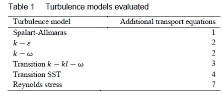
The present work seeks to meet this objective by comparing the results of various numerical simulations in which each of the commonly used RANS turbulence models listed in table 1 are applied - using both standard wall functions and low Reynolds number modelling as appropriate, against experimental data. It is found that the RNG k - ε model with enhanced wall treatment applied gives the most accurate prediction of the near-wall static pressures out of the models considered in the assessment.

 

 

2 Experimental method

An experimental investigation [5] was conducted to measure the streamwise static pressure profile over a surface-mounted hemisphere immersed in turbulent air flow, using the open circuit subsonic wind tunnel housed in the Department of Mechanical and Mechatronic Engineering at Stellenbosch University. The interchangeable test section of the wind tunnel has dimensions of 1.42 m width x 0.655 m height x 2.5 m length.

The test model was fashioned from the plastic ball of a buoyancy valve. Nine equidistant pressure-taps were fitted into the surface of the model, which was subsequently polished using sandpaper and water. The pressure taps were connected to an Endress & Hauser pressure transducer via a Furness selection box. The pressure transducer was in turn connected to a computer via a National Instruments data logger. Following instrumentation, the 150 mm-diameter model was glued to a steel plate positioned 0.345 m above the bottom wall of the test section, behind a wire turbulence grid. The height of the steel plate was specifically chosen to ensure that the model remains above the boundary layer in the test section, which can reach a thickness of up to 0.2 m at high flow velocities [8]. The resultant blockage due to the placement of the hemisphere model in the test section was calculated to be relatively low (approximately 1 %) and correction of the measured free stream velocity was therefore deemed unnecessary. A Pitot-static tube connected to a second pressure transducer was positioned behind the inlet to the test section to measure the free stream pressures. The experimental setup is shown in figure 1.

 

 

During the experiment, static pressure readings were taken from the pressure taps in the test model, and static, stagnation and hence dynamic pressures readings were taken from the Pitot-static tube. At each position three readings each were taken at a sampling rate of 1000 Hz for 5 seconds, nominally at two air flow velocities - 20 m/s and 30 m/s. Sampling of the data received via the data logger was performed using the measurement software VI Logger (Version. 2.0.1 [6]).

 

3 Numerical simulation method

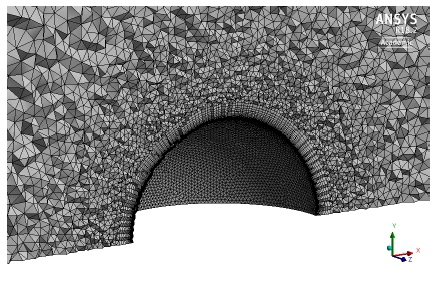
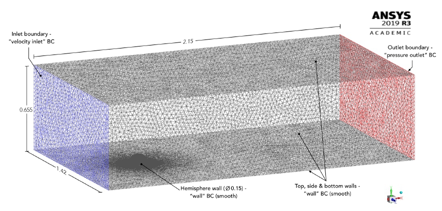
Numerical simulation of the flow was undertaken using the academic version of the commercial CFD software ANSYS Fluent, integrated into ANSYS Workbench 18.2 [7]. Figure 2 shows the computational domain and the specified boundary conditions. While the height and width of the computational domain are identical to that of the wind tunnel, the length of the computational domain was chosen somewhat shorter, at 2.15 m - approximately 10 times the diameter of the model. This has come to be a heuristic commonly used in the literature, as it has been found to ensure that the outlet boundary of the computational domain is positioned just far enough from the hemisphere to capture the entirety of the wake, but close enough to avoid expending computational time and resources solving the transport equations on a subregion of the domain that has no bearing on the solution. The mesh for the bulk of the computational domain was generated using tetrahedral cells, and inflation layers comprised of rectangular cells were used at the hemisphere wall, where the largest velocity gradients are anticipated. A body sizing with a soft maximum element size constraint of 3 was applied on the bulk mesh, and a face sizing with a soft maximum element size constraint of 2.5 mm was applied on the hemisphere wall. The height of the first layer of inflation cells was estimated based on the y⁺value required to implement the near-wall modelling approach, as discussed shortly. The number of inflation layers and the growth rates on the face and body sizings were then chosen to facilitate a smooth transition in the size and aspect ratio of the cells from the hemisphere wall to the bulk mesh, as shown in figure 3.

 

 

A variety of near-wall modelling methods are supported in ANSYS Fluent, such as standard wall functions, resolving the viscous sublayer, and an enhanced wall treatment method designed to use either one or both the aforementioned approaches, depending on the local mesh parameters. In some cases, the implementation of a turbulence model in ANSYS Fluent supports more than one approach, depending on the theoretical formulation of the model. Which method to use is then a question of the nature of the flow being simulated, the available time and computational resources, and the desired accuracy of the solution.

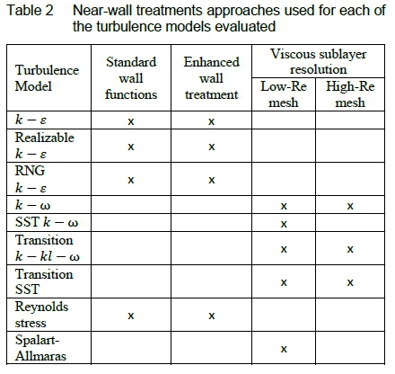
Simulations were carried out using each of the three near-wall modelling methods mentioned above, for all wall boundaries (figure 2), as summarised in table 2. Accordingly, two mesh variants were created - a "high Reynolds number mesh" for use with standard wall functions and a "low Reynolds" number mesh for use with the enhanced wall treatment option, the primary difference between the two being the first layer height (4.58-10"⁴ m for the former and 1 · 10^-5 m for the latter, corresponding to y⁺ < 1 and 30 < y⁺ < 300, respectively) and the number of inflation layers (10 and 30 layers respectively). Both mesh variants were used for resolution of the viscous sublayer, as indicated in table 2.

 

 

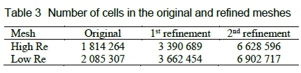
Grid independence was demonstrated by reducing the maximum cell size to 2 cm in the first stage of refinement, and once again to 1.5 cm. Grid adaptation was enabled to allow additional refinement or coarsening of the cells near the hemisphere wall during the solution process, once after 100 iterations, and again after 200 iterations, to ensure the y+ values remained in the specified range. The number of cells in the original and refined meshes, prior to adaptation, are shown in table 3. No significant changes in the predicted static pressure profiles were noted with the successive refinements to the mesh.

 

 

The level of turbulence in the flow is imputed from model-specific scalar properties (e.g. turbulence kinetic energy, turbulence dissipation rate) which are assigned values at the domain inlet based on measurements. The calculation of the boundary values is based on knowledge of the turbulence intensity I, for which empirical relations were derived by Combrinck [8], whose experimental setup is replicated in the present work. This approach is reasonable since the elevation of the hemisphere above the boundary layer along the floor of the wind tunnel test section ensures uniformity of the inlet velocity profile.

The simulations were solved using the pressure-based solver in ANSYS Fluent [7], utilising the SIMPLE pressure-velocity coupling scheme. The Green-Gauss Node-Based gradient evaluation scheme was applied for the momentum equation and the second-order upwind scheme applied for all other transport equations, with no changes to the default under-relaxation factors. Specifying the flow velocity and the corresponding values of the relevant turbulence quantities at the inlet boundary, the solutions were then initialised and allowed to iterate. The simulations carried out on the high Reynolds number mesh were allowed 2500 iterations and those using the low Reynolds number mesh allowed 5000 iterations, although the flow parameters generally converged about their respective mean values before these limits were reached.

 

4 Results

The results of the wind tunnel experiment and the numerical simulation are presented and compared below, with the pressure coefficient profile along the centreline of the hemisphere serving as the main evaluation metric. The pressure coefficients are found to be nearly identical for free stream velocities of 20 m/s and 30 m/s in both the experimental and numerical analysis. Consequently, the experimental and numerical results are only compared for the case of 20 m/s free stream velocity.

4.1 Experimental results

The static pressures measured in the wind tunnel experiment were converted to pressure coefficients, plotted on figure 4 below. The maximum and minimum pressures correctly indicate the expected approximate locations of the stagnation point and the onset of the adverse pressure gradient at a = 15° and a = 65° respectively. Separation of the surface shear layer from the wall of the model occurs in the region of a = 130°. It should be noted that due to the limited number of pressure taps, the profiles shown are crude, and the locations of the pressure extrema and separation points are only approximate.

 

 

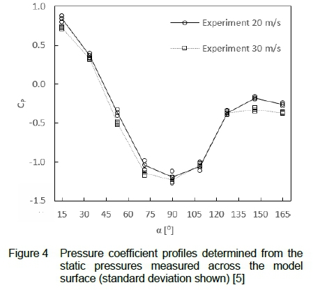
The experiment by Combrinck [8] was conducted for similar flow conditions using a model of identical size to that used in the present work. The data shown in figure 4 correlate well with those of Combrinck [8] (figure 5), except for two notable differences at the fifth and sixth pressure tapping points (a = 90° and a = 110°), with which Combrinck reported having issues during the experimental campaign. Apart from slight differences, the pressure coefficients calculated from the static pressure readings taken at 20 m/s and 30 m/s free stream velocity exhibit no significant differences. This is confirmed by the data reported by Combrinck, and, considering the diameter-based Reynolds numbers of Re = 2.05 x 10⁵ and Re = 3.08 x 10⁵ calculated for airflow of 20 m/s and 30 m/s respectively, supports the conclusion of Cheng et al. [9] that the pressure distributions become independent of the Reynolds number for Re > 2.0 x 10⁵. A slight difference is noted between the absolute values of the experimental pressure coefficients for 20 m/s free stream velocity (Re = 2.05 x 10⁵) and those obtained by Cheng et al. [9] for Re = 2.06 x 10⁵ (figure 5).

 

 

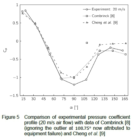
The trend, however, is the same and the difference is likely caused by differences in the level of incoming boundary layer and turbulence intensity in the two experiments. A similar offset was noted by Tavakol et al. [2] in the results of their experiments. A detailed description of the influence of the incoming boundary layer and turbulence intensity on the pressure distribution along the streamwise centreline of a hemisphere is given by Savory and Toy [10].

The experimental results are thus concluded to compare well with the results of similar experiments described in the literature and are considered an adequate basis for the subsequent assessment of the numerical results.

4.2 CFD results

4.2.1 Results of simulations using the high Reynolds number mesh

Figure 6 shows the predicted pressure coefficient profiles obtained using standard wall functions with the applicable subset of the turbulence models. The predictions of the simulations show good agreement with the experimental data up to oc« 65°, after which the adverse pressure gradient sets in and the simulation results begin to deviate from the experimental results, continuing into the separation region in the near wake behind the hemisphere.

 

 

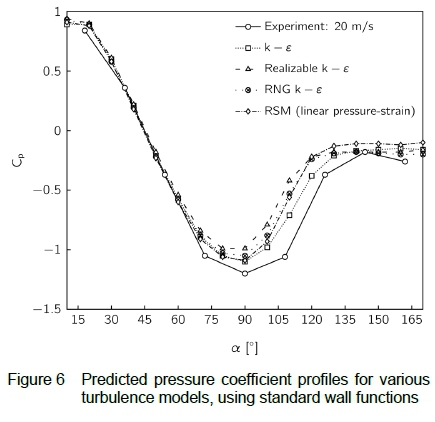
Disagreement between the numerical and experimental results in this region of the model is in line with theoretical expectations since the standard wall-function approach assumes a perfectly flat surface about which the flow has a favourable pressure gradient. Figure 7 shows the predicted pressure coefficient profiles obtained by resolving the boundary layer flow on the high Reynolds number mesh and using the applicable subset of the turbulence models. The Transition k - kl - ω shows close agreement with the experimental data along much of the hemisphere wall, predicting the acceleration of the flow at the apex with good accuracy, but significantly overestimating the pressure in the separation zone on the leeward side of the hemisphere.

 

 

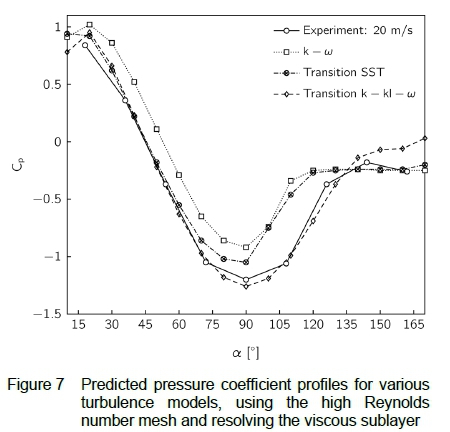
The Transition SST model predicts the flow with accuracy comparable to that of the models using standard wall functions, and the k - ω model is found to yield the least accurate prediction, with a mean error of 26.58 %.

4.2.2 Results of simulations using the low Reynolds mesh

The accuracy of the pressure coefficient predictions is generally found to improve when enhanced wall treatment is applied or the viscous sublayer is resolved on the low Reynolds number mesh, as shown in figures 8 and 9.

 

 

 

 

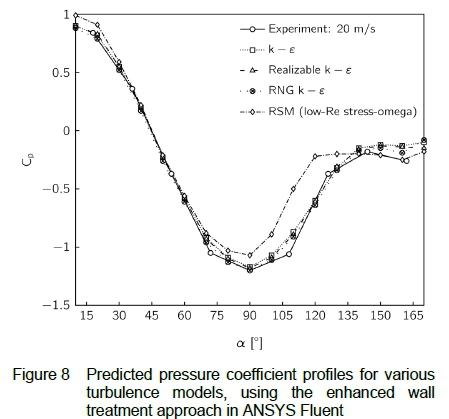
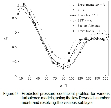
Comparing figures 6 and 8 shows that the predictions of the k - ε model and its variants are considerably more accurate when enhanced wall treatment is used. This stands in contrast with the predictions of the Reynolds Stress model and k - ω model, in which changing the near-wall modelling approach is found to bring about little improvement. The Spalart-Allmaras and Transition k - kl - ω model show good agreement with the experimental data, suggesting that the sampling rate used in the experiment, and the subsequent pooling of the data, allowed adequate capturing of the local pressure and velocity fluctuations near the pressure tapping points.

It must be noted that these results pertain to the steady state solution of a flow problem that is in fact time-dependent and that consequently, the absolute accuracy of the predictions yielded by the various turbulence models can possibly be improved if time-dependent solutions are sought.

Nevertheless, the given comparison of the relative accuracy with which the various turbulence models give approximate steady state predictions reveals that the approximate results of a steady state simulation may be satisfactory for some investigations, for instance, for preliminary study, at relatively low computational expense, prior to a comprehensive time-dependent simulation.

Given that the accuracy of the single-equation Spalart-Allmaras model is comparable to that of the 2-equation RNG k - ε model and the 3-equation Transition k - kl - ω model, it is recommended that a future investigation compare the accuracy of their time-dependent solutions to assess whether any improvement is gained from the additional computational demand of the latter for this class of flows.

Further analysis was undertaken in which the spanwise velocity distribution at various streamwise positions behind the hemisphere, and the velocity profile in the streamwise symmetry plane were evaluated. The velocity profiles were found to agree with theoretical expectations and data from the literature [2], thus supporting the validity of the numerical results.

 

5 Conclusion

A suitability assessment of different turbulence models was conducted for the case of flow over a smooth surface-mounted hemisphere, comparing the steady flow solutions of numerical simulations performed using six common RANS turbulence models and a variety of near-wall modelling approaches against experimental data.

Using pressure coefficients at different streamwise locations along the surface of the hemisphere as the primary metric, it is found that the RNG k - ε model with enhanced wall treatment applied predicts the pressure coefficient profiles most accurately with a mean error of 4.83 %, and is therefore considered to be the optimal turbulence model for the flow in question. The Reynolds Stress model and the standard k - ω model were found to give the least accurate predictions, regardless of the near-wall modelling approach applied. Interestingly, the single-equation equation Spalart-Allmaras model was found to show very good agreement with the experimental data - comparable to the predictions of the 2-equation RNG k - ε and 3-equation Transition k - kl - ω models, with the viscous sublayer resolved on a low Reynolds number mesh in each case. Another interesting observation is the relatively good accuracy with which the Transition k - kl - ω model predicts the pressure coefficient profile when the boundary layer is solved on a high Reynolds number mesh.

These findings emphatically demonstrate that additional complexity need not guarantee greater accuracy. The results also suggest that while using enhanced wall treatment or resolving the viscous sublayer yields on a low Reynolds number mesh generally give superior predictions, using standard wall functions with an appropriate turbulence model can yield usable accurate results on the windward side of the hemisphere surface which may be adequate for simulations focused on this region of the flow.Although the findings presented here stem from simulations of flow past a smooth protuberance, the insights afforded may be of use to CFD practitioners requiring a turbulence model suitable for simulating such flows when the use of a low Reynolds number mesh would be prohibitive due to large variations in the size and distribution of roughness elements. Thus, it is recommended that the effects of surface roughness on the suitability of various turbulence models for this case of flows be thoroughly assessed in future research.

 

Acknowledgement

Computations were performed using the University of Stellenbosch's HPC1 (Rhasatsha): http://www.sun.ac.za/hpc

 

References

[1] M. M. Tavakol and M. Yaghoubi. Experimental and numerical analysis of turbulent air flow around a surface mounted hemisphere. Transaction B: Mechanical Engineering, 17(6):480-491, 2010.         [ Links ]

[2] M. M. Tavakol, M. Yaghoubi and M. M. Motlagh. Air flow aerodynamic on a wall-mounted hemisphere for various turbulent boundary layers. Experimental Thermal and Fluid Science, 34(5):538-553, 2010.         [ Links ]

[3] R. N. Meroney, C. W. Letchford and P. P. Sarkar. Comparison of numerical and wind tunnel simulation of wind loads on smooth, rough and dual domes immersed in a boundary layer. Wind and Structures 5(2):347-358, 2002.         [ Links ]

[4] P. Enshaie, J. McCarthy, M. Giacobello and B. Thornber. Suitability of different numerical models for simulating flow over a hemispherical protuberance. Proceedings of the 21^st Australasian Fluid Mechanics Conference, Adelaide, Australia, 10-13 December 2018.

[5] J. F. Bruwer. Determination of the Optimal Turbulence Model for the Numerical Analysis of Turbulent Air Flow Around a Surface Mounted Hemisphere. Capstone Project Report, Department of Mechanical and Mechatronic Engineering, Stellenbosch University, South Africa, 2012.

[6] National Instruments Corporation. VI Logger User Guide, 2004.

[7] ANSYS Inc. Fluent in Workbench User Guide, Release 18.2, 2017.

[8] M. L. Combrinck. A Computational Fluid Dynamic Analysis of the Airflow Over the Keystone Plant Species, Azorella Selago, on Subantarctic Marion Island. MScEng thesis, Department of Mechanical and Mechatronic Engineering, Stellenbosch University, South Africa, 2008. URL: http://hdl.handle.net/10019.1/2314        [ Links ]

[9] C. M. Cheng, C. L., Fu and Y. Y. Lin. Characteristic of wind load on a hemispherical dome in smooth flow and turbulent boundary layer flow. Bluff Bodies Aerodynamics and Applications, Milano, Italy, 20-24 July 2008.

[10] E. Savory and N. Toy. Hemispheres and hemisphere- cylinders in turbulent boundary layers. Journal of Wind Engineering and Industrial Aerodynamics, 23:345-364, 1986.         [ Links ]

 

 

Received 6 November 2019
Revised form 8 October 2021
Accepted 12 October 2021