ARTICLES
http://dx.doi.org/10.17159/2309-8988/2021/v37a5

 

Performance Enhancement of an Induced Draught Axial Flow Fan Through Pressure Recovery

 

 

G. M. Bekken^I; C. J. Meyer^II; S. J. van der Spuy^III

^IPhD Candidate. Department of Mechanical and Mechatronic Engineering, Stellenbosch University, South Africa. E-mail: 17732956@sun.ac.az
^IIAssociate Professor. Department of Mechanical and Mechatronic Engineering, Stellenbosch University, South Africa. E-mail: cjmeyer@sun.ac.za
^IIISAIMechE Member, Professor. Department of Mechanical and Mechatronic Engineering, Stellenbosch University, South Africa. E-mail: sjvdspuy@sun.ac.za

 

 

---

ABSTRACT

This study illustrates that downstream diffusers can significantly aid the performance of an induced draught axial flow fan. Two conical diffusers of length 0.2 and 0.4 times the fan diameter and an annular diffuser with a length equal to the fan diameter are tested. At the design flow rate of the fan, the short conical diffuser increases the available static pressure by 17.6 % and the static efficiency by 8.9 %. The medium-length conical diffuser increases it by 21.9 % and 11.7 %, respectively. The long annular diffuser produces a 28.2 % pressure increase and a 14.2 % efficiency increase. The paper also compares the obtained pressure recovery coefficients of the different discharge diffusers using two-dimensional axisymmetric and three-dimensional computations. It shows that the pressure at the outlet of the fan cannot be assumed to be equal to atmospheric pressure, as is prescribed by the fan testing standards. A new method of measuring pressure recovery from two-dimensional computations is proposed.

Additional keywords: Pressure recovery, axial flow fan, diffuser.

---

 

 

Nomenclature Roman

A Cross-sectional area [m²]

C_D Drag coefficient

C_L Lift coefficient

c Absolute velocity [m/s]

c_h Chord length [m]

d Diameter [m]

F Force [N]

K_recPressure recovery coefficient

Modified pressure recovery coefficient

k Turbulence kinetic energy [m²/s²]

L Characteristic length [m]

I Length [m]

Ρ Power consumption [W]

ρ Pressure [Pa]

r Radius [m]

t Actuator disc thickness [m]

U Velocity [m/s]

V Volume [m³]

V Volume flow rate [m³/s]

ν Mean axial velocity [m/s] y Wall-normal distance [m]

y⁺ Sublayer-scaled wall-normal distance

Greek

a_att Angle of attack [deg]

β Relative flow angle [deg]

ft Turbulence model constant, 0.075

Δ Differential

δ Per computational cell

η Efficiency [%]

θ Diffuser half-wall angle [deg]

ν Kinematic viscosity [m²/s]

v_t Turbulent kinematic viscosity [m²/s]

ρ Air density [kg/m³]

σ Blade solidity

ω Turbulence specific dissipation rate [s^-1]

Subscripts

clear Axial clearance

d Dynamic pressure

dif Diffuser

dump Dump representing the open atmosphere

e Exit (fan outlet)

F Fan

FC Fan casing

F/dif Fan-diffuser unit

FH Fan hub

i Inner diffuser wall

inlet Inlet boundary

o Outer diffuser wall

plen Plenum chamber upstream of fan

R Relative

s Static pressure

tip Fan blade tip

χ, θ Axial and tangential directions

∞ Atmospheric or free-stream conditions

Abbreviations

2D, 3D Two- and three-dimensional

ADM Actuator disc model

CFD Computational fluid dynamics

DIC Diagonal-based incomplete Cholesky smoother

DILU Diagonal-based incomplete LU preconditioner

GAMG Geometric agglomerated algebraic multigrid solver

P3D Periodic three-dimensional model

PBiCG Preconditioned bi-conjugate gradient solver SIMPLE

Semi-implicit method for pressure-linked equations

SST Shear-stress transport

 

1 Introduction

In the power plant cooling industry, it is accepted that exhaust diffusers can aid the performance of induced draught axial flow fans. However, there is a lack of concrete recommendations as to which diffuser configuration (conical or annular) would be best, how long the diffuser should be, or which divergence angles are best. Kröger [1] states that practical diffusers normally have included angles in the range of 12° < 2θ < 17°. Eck [2], on the other hand, argues that it is impossible to provide exact rules for diffuser diffusion angles: Although half-wall angles in the range of 7° < θ < 9° are often recommend, better diffuser performance might be obtained within the wider range of 5° < θ < 20°, depending on the Reynolds number and turbulence quantities.

Diffuser design charts with recommended diffusion angles exist: Wallis [3] provides charts for two-dimensional, conical, and annular diffusers. McDonald and Fox [4] provide a chart for conical diffusers, and Sovran and Klomp [5] provide one for annular diffusers. Generally, the data in these charts were obtained using uniform inlet flow conditions that are swirl-free. However, swirl is present at the outlet of an axial flow fan. The velocity profiles that will enter the downstream diffuser will thus be non-uniform. Kröger [1] therefore states that such diffuser design charts can at best provide only approximate performance characteristics.

Furthermore, it is generally accepted that modest levels of swirl at the inlet of a diffuser can be beneficial for its performance [3]. That is because swirl energizes the near-wall flow, delaying the onset of stall. McDonald et al. [6] as well as Neve and Wirasinghe [7] found that wide-angled diffusers that would normally have stalled under uniform inlet flow conditions significantly benefited from inlet swirl. The inlet swirl had a forced-vortex distribution. They also found that the performance of the diffusers improved with increasing swirl up to a point, whereafter the performance deteriorated sharply. The drop in performance is due to a rotating core which forms as a result of excessive swirl. Senoo et al. [8] and Okio et al. [9] obtained similar results for conical diffusers using a Rankin-vortex inlet swirl distribution. Moreover, Kumar and Kumar [10], Singh et al. [11], and Mohan et al. [12] obtained similar findings for annular diffusers. For conical diffusers, Senoo et al. [8] made the point that there exists an optimum diffuser opening angle with a corresponding optimum level of inlet swirl. Likewise, for annular diffusers, Kumar and Kumar [10] found that the optimum level of swirl is specific to a particular diffuser geometry. Mohan et al. [12] also found that the shorter and wider the discharge diffuser, the more swirl is needed to improve its performance and the more sensitive the performance becomes to the degree of inlet swirl.

Walter et al. [13] attempted to determine how pressure recovery could improve the performance of an induced draught axial flow fan. Pressure recovery refers to the amount of dynamic pressure that would normally be lost at the outlet of the fan that can be converted to static pressure. It can be achieved with downstream diffusers, stator blade rows, or both. Walter et al. [13] demonstrated that the static efficiency of the fan could be increased by 7 % at a typical design point using a downstream stator blade row. Adding an annular diffuser to the fan-stator unit can increase the efficiency by a further 20 %. These are substantial gains in performance. However, this study was purely based on theory. No experiments or numerical work were done to substantiate the findings.

Bekker et al. [14] investigated pressure recovery for an induced draught axial flow fan. They tested various discharge configurations which included a downstream stator blade row, conical and annular diffusers with and without stators at their inlets, and an annular diffuser with a stator row at its outlet. They found that an annular diffuser of length equal to the fan diameter having equiangular walls directed 22° from the axial direction recovered the most pressure over a range of flow rates for the M-fan of Wilkinson et al. [15]. With this diffuser, the operating point of the M-fan shifted to a 6.3 % higher flow rate and 20 % higher static efficiency compared to the initial design point of the fan.

From the above literature, it is clear that finding the optimum diffuser for a particular application is highly problem-specific: inlet flow uniformity, swirl distribution, and swirl intensity all influence optimum diffuser performance. For fan application, Kröger [1] therefore suggests that, if possible, the fan and diffuser should be tested together to obtain the combined performance characteristics of the fan-diffuser unit. In this paper, Kröger's [1] advice will be followed: Discharge diffusers of three different lengths will be simulated together with the M-fan of Wilkinson et al. [15] to establish how the diffusers affect the fan's performance. All simulations will be performed using the open-source CFD code, OpenFOAM.

This paper starts by presenting details of the M-fan followed by an explanation of the numerical model that will be used to model the fan. Thereafter, the numerical solution strategies that were used are provided. The axial flow fan model is then validated against experimental and numerical data obtained from other sources. Details concerning two-dimensional axisymmetric computations that were performed for the discharge region of the fan follows. This is followed by three-dimensional computations where the fan and diffusers were modelled together. The pressure recovery data of the two- and three-dimensional simulations are then compared. Finally, the main findings are summarised in the concluding section.

 

2 The M-fan

Wilkinson et al. [15] designed the M-fan to be used in forced draught air-cooled condensers. The fan has eight blades and a hub-to-tip ratio of 0.29. The design blade setting angle is 34° at the hub. In table 1, further design specifications of the fan are listed. Also listed in the table are the specifications of the scaled fan for the BS EN ISO 5801 [16] fan test facility at Stellenbosch University. The fan casing diameter in this facility is 1.542 m. For both fan sizes, the tip speed is Utip = 58 m/s.

 

 

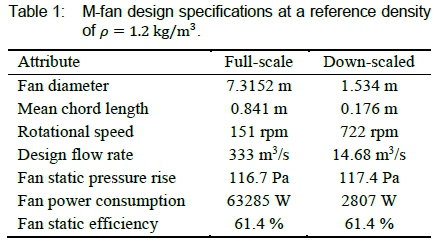
The NASA-LS 0413 aerofoil profile was used as the base profile for the fan blades. However, the aerofoil camber distribution was optimised to maximise the lift-drag ratio along the span of the blade. In other words, the aerofoil profile varies along the blade span.

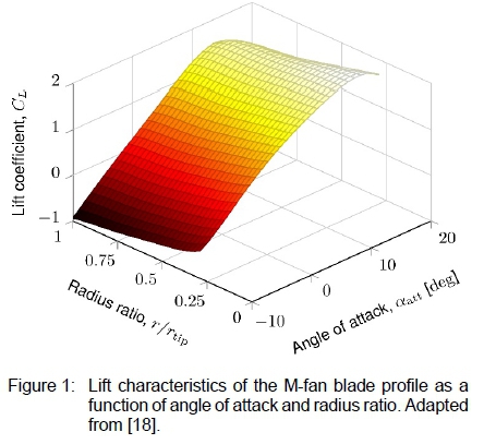
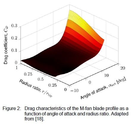
Wilkinson et al. [15] used XFOIL [17] to compute the C_L versus α_att and C_Dversus α_att data at 20 radial stations along the span of the fan blade. At each section, the aerofoil thickness, camber, and chord-based Reynolds number were taken into account. Fifth order surfaces were fitted to the data, allowing for C_Land C_Dto be functions of both the angle of attack and blade span. Figures 1 and 2 depict the lift and drag characteristics, respectively.

 

 

 

 

3 Axial Flow Fan Model

The axial flow fan was modelled using the actuator disc model (ADM) developed by Thiart and Von Backström [19]. The model computes the forces that a fan blade would exert on the air by taking the relative velocity vector and flow angle, blade solidity, and blade profile characteristics into account. The forces are introduced into the Navier-Stokes equations through momentum source terms. The axial component per volume is calculated with

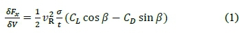
and the tangential component per volume with

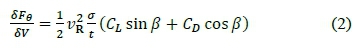
The ADM assumes the radial force to be negligibly small. In the above equations, v_Rand β are the relative velocity vector and flow angle, σ is the blade solidity, and t is the thickness of the actuator disc. Depending on the angle of attack at a specified radial location, the lift and drag coefficients, C_Land C_D, are obtained from the polynomial curves in figures 1 and 2.

The ADM has proved to produce fan performance characteristics in close agreement with experimentally obtained fan data [20]. Wilkinson et al. [15, 21] have successfully employed this particular version of the model which makes use of the lift and drag data presented in figures 1 and 2. However, as a result of the ADM not accounting for radial forces, the model has been found to perform poorly at low flow rates [22].

 

4 Numerical Solution Method

The computational fluid dynamic (CFD) computations were performed using open-source software: OpenFOAM-5.0 was used for the two-dimensional (2D) axisymmetric computations, and the three-dimensional (3D) problems were solved with OpenFOAM-v1906.

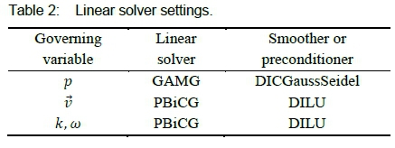
The SIMPLE algorithm was used for pressure-velocity coupling. All gradient terms were discretised using a second-order-accurate linear scheme. Divergence terms for velocity were discretised using a bounded linear-upwind scheme that is second-order accurate. A bounded upwind differencing scheme of first-order accuracy was used for the turbulence divergence terms. The Laplacian terms were discretised using linear interpolation from cell centres to face centres and a limited scheme with a correction coefficient of 0.5 for surface-normal gradients. The resulting linear system of equations was solved iteratively with the linear solvers listed in table 2.

 

 

Air properties at an atmospheric pressure of 101 325 Pa and a temperature of 20 °C were used for all computations. The kinematic viscosity and density were thus ν ~ 1.5χ10"⁵ m²/s and ρ ~ 1.2 kg/m³, respectively. The effects of turbulence on the mean flow were modelled using the k-ω model of Wilcox [23]. Bekker et al. [14] found that this model predicted swirling flow in a conical diffuser with reasonable accuracy.

 

5 Axial Flow Fan Model Validation

The ADM employing the lift and drag data in figures 1 and 2 is validated against experimental fan data. Wilkinson et al. [21] measured the data using the BS EN ISO 5801 fan test facility at Stellenbosch University. It is a type A test facility, meaning the fan has a free inlet and outlet (i.e., not ducted). The fan data were gathered for tip clearances of 2, 4 and 6 mm. The ADM results of Wilkinson et al. [15] for the M-fan will also be included for comparison. They used the same lift-drag curves as in figures 1 and 2, but their simulations were performed utilizing ANSYS FLUENT 17.2.

The computational domain and boundary conditions are depicted in figure 3. Engelbrecht et al. [24] and Wilkinson et al. [15] also used this domain to represent the BS EN ISO 5801 fan test facility. The inlet of the settling chamber was set to have a specified constant volumetric flow rate, and a low turbulence intensity of 3 % was used to compute the turbulence kinetic energy at the inlet. Menter [25] illustrated that the k-ω model is sensitive to the specified inlet ω-value. If the latter is too small, the turbulence viscosity becomes unrealistically large, causing poor velocity profile predictions. Consequently, he recommended ω > 10∞/L, where L is a characteristic length. Spalart and Rumsey [26], on the other hand, obtained corrupted velocity profiles in the boundary layer with excessive ω-values using Menter's [27] shear-stress transport (SST) version of the k-ω model. They obtained realistic results with ωL/U∞ up to 100. Subsequently, an inlet turbulence viscosity ratio of ν/ν = 0.4 was used in combination with the inlet turbulence intensity of 3 % to produce 10 < ω_ch/U∞ < 100 for the range of flow rates tested for the M-fan.

 

 

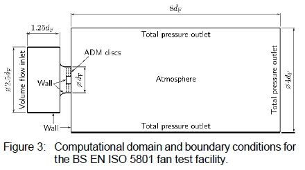
The outlet boundary represents the open atmosphere and a total pressure boundary condition of 101 325 Pa was assigned to it. Velocity and turbulence quantities were set to have zero gradients at the outlet. In the case of reverse flow at the outlet boundary, the velocity was computed from the flux in the patch-normal direction. As depicted in figure 3, the walls of the settling chamber, fan casing, bellmouth and hub, as well as the fan discharge plane were set to wall boundaries. A no-slip condition along with zero gradients for pressure were assigned to these walls. Since the near-wall flow is not of great importance at this stage, wall functions for turbulence kinetic energy and turbulence specific dissipation rate were used to model the near-wall flow.

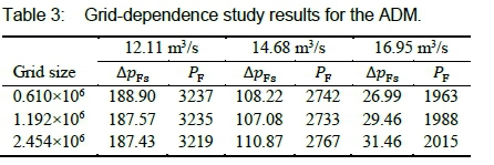
The computational grid was generated with OpenFOAM's blockMesh utility, producing a block-structured mesh comprising of hexahedral elements. The fan's performance was computed at flow rates near the design point on three successively refined meshes. Table 3 illustrates that the fan static pressure prediction of the coarsest mesh is slightly low at the high flow rate. The results of the medium mesh, however, can be considered grid-independent. The mesh with 1.192χ10⁶ cells was thus used for all further computations in this study. The maximum and mean non-orthogonality of the selected mesh was 68.6 and 3.2, respectively. The highest skewness in the mesh was 0.84 and the cell aspect ratio reached 27.2 near solid surfaces.

 

 

Solutions were deemed converged when the fan static pressure and power consumption no longer changed from iteration to iteration. The normalised residuals for the underlying equations reached an order of magnitude ranging between 10^-3 and 10^-4. Pressure, velocity and turbulence variables were under-relaxed with factors of 0.2, 0.3 and 0.3, respectively.

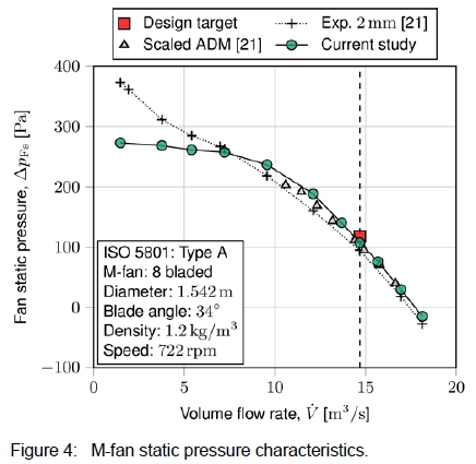
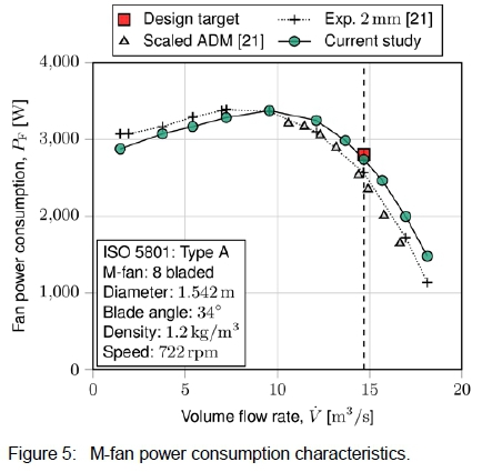
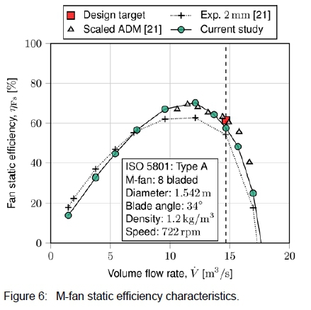
By evaluating the fan performance at a series of inlet volumetric flow rates, the fan characteristic curves were computed. Figures 4, 5 and 6 depict the fan static pressure, power consumption, and static efficiency characteristics, respectively. The ADM's low pressure predictions at low flow rates is a well-known shortcoming of the model, caused by the model's inability to account for radial forces [20, 28]. In the vicinity of the design flow rate, the static pressure and power consumption are higher than the experimental measurements. As noted by Wilkinson et al. [21], the model's slight over predictions are caused by its inability to account for tip clearance losses. Overall, the agreement with the experimental measurements and ADM results of Wilkinson et al. [21] is reasonable.

 

 

 

 

 

 

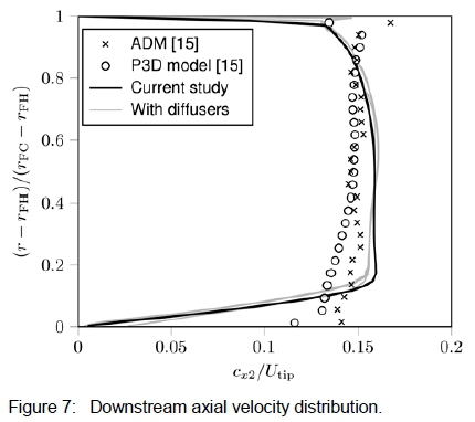
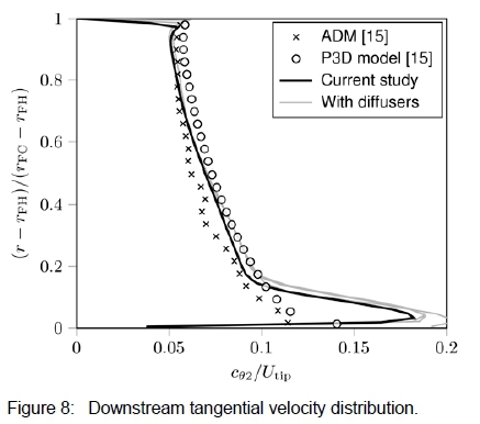
Since Johnston [29] and Wright et al. [30] established that diffuser performance is sensitive to the inlet flow conditions, the ADM needs to predict the fan's downstream velocity profiles accurately. The velocity profiles obtained with the ADM will thus be compared to Wilkinson et al.'s [15] ADM profiles as well as the velocity profiles they measured downstream of a periodic three-dimensional (P3D) model. Figures 7 and 8 provide the axial and tangential velocity profiles at the outlet of the fan, respectively. The figures include the velocity profiles at the outlet of the fan when the diffusers in the following sections were appended to the fan. It serves to illustrate that the addition of the diffusers does not alter the flow in the vicinity of the fan. Although the ADM of this study overestimates the swirl near the hub, the overall agreement with the profiles of Wilkinson et al. [15] is fair.

 

 

 

 

6 2D Downstream Diffuser Simulations

Bekker et al. [14] aimed to find a discharge configuration for the M-fan that produces high pressure recovery coefficients over a range of operating volume flow rates. They considered stator blade rows, conical and annular diffusers, as well as stator-diffuser combinations. However, they only considered a diffuser length equal to the fan diameter. As seen in table 1, fans in air-cooled condensers are large. A diffuser with a length equal to the fan diameter combined with a modest axial clearance between the fan and downstream diffuser would result in an appendage of 8 m or more being added to the M-fan.

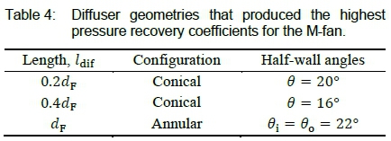
The same procedure as followed by Bekker et al. [14] was thus repeated for two shorter diffuser lengths: Firstly, a length equal to 40 % of the fan diameter, which Kröger [1] terms "practical". Secondly, an even shorter length of 20 % the fan diameter. Table 4 summarises the particulars of the discharge configuration of each length that produced the highest pressure recovery coefficients over a range of volumetric flow rates.

 

 

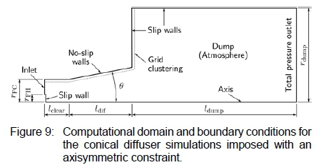
The two-dimensional axisymmetric simulations for the conical diffusers were performed using the wedge-shaped computational domain depicted in figure 9. The wedge angle of the domain was five degrees, as recommended by OpenFOAM's user manual for axisymmetric simulations [31]. The domain used for the annular diffuser was similar. Although, its hub terminated at the outlet of the diffuser and diverged so that the inner and outer walls were parallel.

 

 

The meshes were generated with blockMesh, yielding block-structured meshes with hexahedral elements. Since wall functions are not advisable in adverse pressure gradients [23], grid-clustering was added near solid surfaces to facilitate integration through the boundary layer. The width of the clustered zone was 5 % of the fan radius and had a high degree of grading towards the wall. The grading allowed for y+ ~ 1 at the walls while transitioning smoothly with the interior mesh.

The maximum non-orthogonality of the resulting meshes was below 70 and averaged between five and ten for the different cases in table 4. The maximum mesh skewness for the 0.24f and 0.44? length conical diffusers was 1.8 and 1.9, respectively. For the annular diffuser, the skewness reached 3.5. As a result of the strong grid clustering near the walls, wall-adjacent cells reached aspect ratios in the order of 1000. Although this is very high, such aspect ratios are common in simulations involving integration through the viscous sublayer.

In these axisymmetric computations, only the flow downstream of the M-fan was simulated. The fan itself was not modelled. Hence, the inlet of the computational domain represented the outlet of the fan. Downstream velocity and turbulence profiles for the M-fan at flow rates ranging from 260 to 380 m³/s were obtained from Wilkinson [18]. He generated these profiles using a periodic three-dimensional CFD model. The profiles were subsequently used to specify the inlet velocity and turbulence boundary conditions.

An atmospheric gauge pressure of 0 Pa was specified at the outlet boundary. The velocity had a zero-gradient condition for flow exiting the domain. For flow entering the outlet boundary, the velocity was based on the flux in the patch-normal direction. Turbulence quantities were set to have zero gradients at the outlet. At the walls, the turbulence boundary conditions deduced by Wilcox [32] were used. That is, the turbulence kinetic energy was set to zero and the turbulence specific dissipation rate was computed as ω = 6v/ß₁y². Furthermore, velocity had a no-slip condition and pressure was set to zero-gradient at the wall. Wedge boundary conditions were specified for the front and back planes of the axisymmetric domain. The symmetry axis was given a symmetry boundary condition.

Bekker et al. [14] tested for grid dependence by refining the mesh and for sensitivity to boundary distances by increasing the size of the dump used to represent the open atmosphere. For each sensitivity test, they compared the measured pressure difference between the outlet and the inlet of the domain and they compared velocity profiles inside the diffuser. The solutions to follow were computed using meshes of the same density and the same boundary distances as deemed suitable by Bekker et al. [14].

The axisymmetric simulations were performed using OpenFOAM's steady-state solver for turbulent and incompressible flows, i.e. simpleFoam. The pressure equation was under-relaxed with 0.2, the velocity with 0.6, and turbulence quantities with 0.7. Solutions were deemed converged after the pressure difference between the domain inlet and outlet reached a constant value and the normalised residuals reduced to an order of 10^-5 to 10^-6.

Bekker et al. [14] computed the pressure recovery coefficient according to

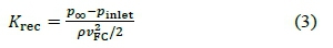
where pinlet was the measured area-weighted static pressure at the inlet of the computational domain and p_∞was equal to atmospheric pressure. The dynamic pressure in the denominator was calculated using the mean axial velocity through the fan casing, v_FC = V/A_FC. This equation was based on the assumption that the pressure at the outlet of the axial flow fan is equal to atmospheric pressure, as specified by the BS EN ISO 5801 standard for type A tests [16]. If no discharge diffuser is present, there should not be any pressure recovery. From equation (3), this implies pintet = so that Krec = 0.

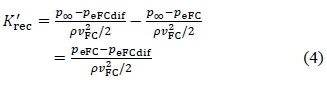
However, the static pressure at the outlet of the fan, p_inet, is indeed not equal to the atmospheric pressure. It is lower than atmospheric pressure. In other words, p_inlet < p∞ will give Krec > 0, even though there is no diffuser present. Equation (3) will thus yield optimistic pressure recovery values. To correct this, a CFD analysis of the fan exit region was performed without any discharge diffuser to determine peFC at various flow rates, i.e. the average static pressure at the fan exit without a diffuser. The same velocity and turbulence profiles of Wilkinson [18] were employed for the analysis. The corrected pressure recovery coefficient, K_rec, can then be obtained by comparing the average static pressure at the fan exit with a diffuser in place, peFCdif, with the average static pressure at the fan exit without a diffuser, peFC. That is,

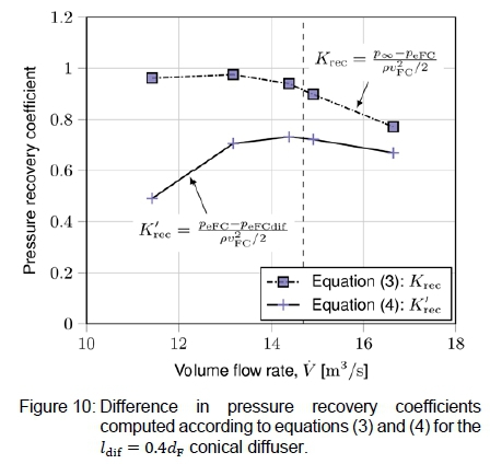
where peFc > peFCdif. Figure 10 illustrates the difference between the pressure recovery coefficients computed using equations (3) and (4) for the ldif = 0.4(¾ conical diffuser. It is clear that equation (3) overestimates the pressure recovery coefficient, especially at low flow rates.

 

 

 

7 3D Fan-diffuser Simulations

In this section, the axial flow fan and diffusers were modelled together to obtain the combined fan-diffuser characteristics. The combined pressure characteristics can then be compared with the pressure characteristics of the fan to determine the pressure recovery coefficients according to

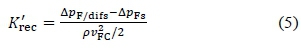
where Δp_F/_difs is the static pressure rise of the fan-diffuser unit and Δp_Fs is the fan static pressure. The latter was defined in accordance with BS EN ISO 5801 for type A tests, viz.,

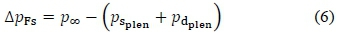
where p∞ is the atmospheric pressure, p_Splen is the static pressure in the plenum chamber (chamber upstream of the test fan), and p_dplen is the dynamic pressure in the plenum chamber. The static pressure rise of the fan-diffuser units, Δp_F/_difs, was also measured as in equation (6).

The same computational domain, boundary conditions, and solution strategy as in section 5 were used. However, the three diffusers of different length were appended to the fan each time. The near-wall treatment for turbulence also differed. As mentioned previously, wall functions generally do not hold in adverse pressure gradients. Therefore, the boundary layer was resolved by adding 11 inflation layers to the walls with snappyHexMesh. The cell layer adjacent to the wall was refined further to ten cell layers using the refineWallLayer utility. This refinement procedure allowed for y+ < 1 at solid surfaces. However, the cell layer addition reduced the quality of the mesh in section 5: Some cells had non-orthogonality of approximately 80 and the average non-orthogonality rose from 3.2 to ~5.

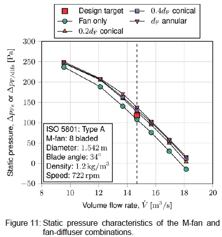
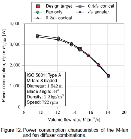
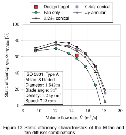
The performance characteristics of the fan-diffuser units are displayed in figures 11 to 13. Figure 11 illustrates that by adding the diffusers, the pressure rise went from slightly below the initial design target of the fan to a pressure rise above that. At the design flow rate, the static pressure rise achieved with the ldif = 0.2(d_f conical diffuser was 17.6 % higher relative to the pressure rise obtained with the ADM for the fan only. The ldif = 0.4(d_f conical diffuser increased the pressure characteristic at the design flow rate by 21.9 % and the ldif = dF annular diffuser increased it by 28.2 %. Figure 12 illustrates that the power characteristics of the fan are essentially unaffected by the added diffusers. Figure 13 then illustrates that the short conical diffuser increased the static efficiency from 57.5 % to 66.4 %, the medium-length conical diffuser increased it to 69.1 %, and the long annular diffuser to 71.7 %.

 

 

 

 

 

 

By subtracting the pressure characteristics of the fan from that of the fan-diffuser units, the pressure recovery coefficients were obtained according to equation (5). Figures 14 to 16 contain the pressure recovery data for the different diffuser lengths. The pressure recovery data obtained with equation (4) for the two-dimensional axisymmetric computations are included for comparison.

 

 

 

 

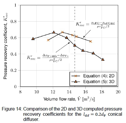
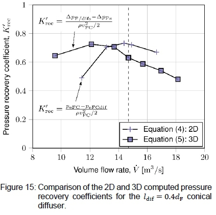
Near the design flow rate, the correlation between the two- and three-dimensional pressure recovery results is fair. In general, the 3D computations yield a recovery coefficient of approximately 0.1 lower than the 2D computations at the design flow rate. At lower flow rates, the 3D results are greater than the 2D results, and at higher flow rates the 3D results are lower. The two- and twee-dimensional pressure recovery coefficients of the conical diffusers in figures 14 and 15 correlate better than that of the annular diffuser in figure 16.

 

 

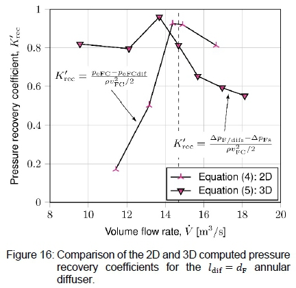
The discrepancies between the two- and three-dimensional pressure recovery data could be due to various factors: Firstly, the 2D simulations were performed for the full-scale fan of 7.3152 m diameter, whereas the 3D computations were for the scaled 1.534 m fan. Since the chord based Reynolds numbers differ for the different fan sizes, the level of turbulence behind the fans will also differ. Secondly, the periodic three-dimensional model of Wilkinson et al. [15] modelled the flow around the physical fan blade. There would thus be a boundary layer at the blade and a wake downstream of the blade. With the ADM, the blades are not physically present. There are thus no boundary layers or downstream wakes caused by the fan blades. In other words, the turbulence levels measured downstream of the ADM will differ from the averaged turbulence data of Wilkinson et al. [15]. Thirdly, the velocity profiles in figures 7 and 8 correlate well with Wilkinson et al. 's [15] data, but they are not exactly the same. The slight difference in the profiles may influence diffuser performance. Fourthly, as mentioned earlier, the ADM generally does not produce accurate results at lower flow rates. This may be the reason for the inconsistencies in the pressure recovery coefficients at the lower flow rates.

 

8 Conclusions

In this paper, the M-fan of Wilkinson et al. [15] was modelled using actuator disc theory. The fan model was validated against experimental measurements and numerical results obtained from other sources. Three different discharge diffusers were added to this fan aiming to improve the performance of the fan through pressure recovery. The first was a conical diffuser with a length equal to 20 % of the fan diameter. The second was 0.4 fan diameters long and also conical. The third and longest diffuser was annular with a length equal to the fan diameter.

Axisymmetric computations were performed for the downstream section of the fan. From these, the pressure recovery coefficients of the diffusers could be computed at various volumetric flow rates. The fan and diffusers were also simulated together in three-dimensional computations to obtain the combined characteristics of the fan-diffuser units. The pressure recovery coefficients of the diffusers were also computed from these results and compared to the axisymmetric results. It revealed that if the pressure at the outlet of the fan is assumed to be equal to atmospheric pressure, as prescribed by the fan test standards, it results in optimistic pressure recovery coefficients. Therefore, a new method of measuring pressure recovery coefficients from axisymmetric computations was proposed.

From the three-dimensional computations, it was found that the ldif = 0.2(d_F conical diffuser increased the available static pressure from 107.36 Pa to 126.23 Pa, i.e. a 17.6 % relative increase. The static efficiency rose from 57.5 % to 66.4 %, an 8.9 % absolute increase. The ldif = 0.44? conical diffuser increased the static pressure by 21.9 % (relative) and the efficiency by 11.7 % (absolute). With the ldif = ¡4 annular diffuser, the available pressure was 28.2 % higher and the static efficiency was 14.2 % higher than it was with the fan alone at the design flow rate.

 

References

[1] D. G. Kröger. Air-cooled heat exchangers and cooling towers: Thermal-flow performance evaluation and design. Department of Mechanical Engineering, Matieland, 1998.

[2] B. Eck. Fans: Design and operation of centrifugal, axial- flow and cross-flow fans. Pergamon Press, 1973.

[3] R. A. Wallis. Axial flow fans and ducts. John Wiley & Sons, 1983.

[4] A. T. McDonald and R. W. Fox. An experimental investigation of incompressible flow in conical diffusers. International Journal of Mechanical Sciences, 8(2):125- 139, 1966.         [ Links ]

[5] G. Sovran and E. Klomp. Experimentally determined optimum geometries for rectilinear diffusers with rectangular, conical or annular cross-section. In G. Sovran (editor), Fluid mechanics of internal flow: Proceedings of the symposium on the fluid mechanics of internal flow, General Motors Research Laboratories, Warren, Michigan, 1965, pp. 270-319. Elsevier, 1967.

[6] A. T. McDonald, R. W. Fox and R. V. Van Dewoestine. Effects of swirling inlet flow on pressure recovery in conical diffusers. AIAA Journal, 9(10):2014-2018, 1971.         [ Links ]

[7] R. S. Neve and N. E. A. Wirasinghe. Changes in conical diffuser performance by swirl addition. The Aeronautical Quarterly, 29(3):131-143, 1978.         [ Links ]

[8] Y. Senoo, N. Kawaguchi and T. Nagata. Swirl flow in conical diffusers. Bulletin of JSME, 21(151):112-119, 1978.         [ Links ]

[9] C. B. Okhio, H. P. Horton and G. Langer. Effects of swirl on flow separation and performance of wide angle diffusers. International Journal of Heat and Fluid Flow, 4(4):199-206, 1983.         [ Links ]

[10] D. S. Kumar and K. L. Kumar. Effect of swirl on pressure recovery in annular diffusers. Journal Mechanical Engineering Science, 22(6):305-313, 1980.         [ Links ]

[11] S. N. Singh, D. P. Agrawal, R. N. Sapre and R. C. Malhotra. Effect of inlet swirl on the performance of wide-angled annular diffusers. Indian Journal of Engineering and Materials Science, 1:63-69, 1994.         [ Links ]

[12] R. Mohan, S. N. Singh and D. P. Agrawal. Optimum inlet swirl for annular diffuser performance using CFD. Indian Journal of Engineering and Materials Science, 5:15-21, 1998.         [ Links ]

[13] J. Walter, S. Caglar and M. Gabi. Investigation of the maximum static efficiency of axial fans. In International Conference of Fan Noise, Aerodynamics, Applications and Systems, Darmstadt, Germany, 2018.

[14] G. M. Bekker, C. J. Meyer and S. J. Van der Spuy. Numerical investigation of pressure recovery for an induced draught fan arrangement. R & D Journal of the South African Institution of Mechanical Engineering, 36:19-28, 2020.         [ Links ]

[15] M. B. Wilkinson, S. J. Van der Spuy and T. W. Von Backström. The design of a large diameter axial flow fan for air-cooled heat exchanger applications. In ASME Turbo Expo 2017: Turbomachinery Technical Conference and Exposition, Charlotte, NC, USA, 2017.

[16] BS EN ISO 5801. Industrial fans - Performance testing using standardized airways. British Standard Institution, 2008.

[17] M. Drela. XFOIL: An analysis and design system for low Reynolds number airfoils. In Low Reynolds number aerodynamics. Springer, 1989.

[18] M. B. Wilkinson. The design of an axial flow fan for air-cooled heat exchanger applications. Master's Thesis, Department of Mechanical and Mechatronic Engineering, Stellenbosch University, 2017.         [ Links ]

[19] G. D. Thiart and T. W. Von Backström. Numerical simulation of the flow field near an axial flow fan operating under distorted inflow conditions. Journal of Wind Engineering and Industrial Aerodynamics, 45(2):189-214, 1993.         [ Links ]

[20] C. J. Meyer and D. G. Kröger. Numerical simulation of the flow field in the vicinity of an axial flow fan. International Journal for Numerical Methods in Fluids, 36(8):947-969, 2001.         [ Links ]

[21] M. B. Wilkinson, S. J. Van der Spuy and T. W. Von Backström. Performance testing of an axial flow fan designed for air-cooled heat exchanger applications. In ASME Turbo Expo 2018: Turbomachinery Technical Conference and Exposition, Oslo, Norway, 2018.

[22] M. B. Wilkinson, F. G. Louw, S. J. Van der Spuy and T. W. Von Backström. A comparison of actuator disc models for axial flow fans in large air-cooled heat exchangers. In ASME Turbo Expo 2016: Turbomachinery Technical Conference and Exposition, Seoul, South Korea, 2016.

[23] D. C. Wilcox. Turbulence Modeling for CFD. 2^nd ed. DCW Industries, 1998.

[24] R. A. Engelbrecht, C. J. Meyer and S. J. Van der Spuy. Modelling strategy for the analysis of forced draft air-cooled condensers using rotational fan models. Journal of Thermal Science and Engineering Applications, 11(5):051011, 2019.         [ Links ]

[25] F. R. Menter. Influence of freestream values on k-w turbulence model predictions. AIAA Journal, 30(6):1657-1659, 1992.         [ Links ]

[26] P. R. Spalart and C. L. Rumsey. Effective inflow conditions for turbulence models in aerodynamic calculations. AIAA Journal, 45(10):2544-2553, 2007.         [ Links ]

[27] F. R. Menter. Two-equation eddy-viscosity turbulence models for engineering applications. AIAA Journal, 32(8):1598-1605, 1994.         [ Links ]

[28] S. J. Van der Spuy. Perimeter fan performance in forced draught air-cooled steam condensers. PhD Thesis, Department of Mechanical and Mechatronic Engineering, Stellenbosch University, 2011.         [ Links ]

[29] I. H. Johnston. The effect of inlet conditions on the flow in annular diffusers. Technical Report, National Gas Turbine Establishment, 1953.

[30] J. R. Wright, B. A. Russel and R. A. Wallis. Annular diffuser studies with 36 in. axial flow fan rig in exhaust configuration, (boss ratio 0.5, area ratios 3.5 and 1.33). Internal Report 71, CSIRO Division of Mechanical Engineering, 1970.

[31] C. J. Greenshields. OpenFOAM: User Guide. 5^th ed. OpenFOAM Foundation Ltd., 2017.

[32] D. C. Wilcox. Reassessment of the scale-determining equation for advanced turbulence models. AIAA Journal, 26(11):1299-1310, 1988.         [ Links ]

 

 

Received 8 December 2020
Revised form 8 April 2021