ARTICLES

 

Numerical Investigation of Pressure Recovery for an Induced Draught Fan Arrangement

 

 

G. M. Bekker^I; C. J. Meyer^II; S. J. van der Spuy^III

^IPhD (Mechanical Engineering) Candidate. Department of Mechanical and Mechatronic Engineering, Stellenbosch University, South Africa. E-mail: 17732956@sun.ac.az
^IIAssociate Professor. Department of Mechanical and Mechatronic Engineering, Stellenbosch University, South Africa. E-mail: cjmeyer@sun.ac.za
^IIISAIMechE Member, Associate Professor. Department of Mechanical and Mechatronic Engineering, Stellenbosch University, South Africa. E-mail: sjvdspuy@sun.ac.za

 

 

---

ABSTRACT

This study investigates the potential gain in operating volume flow rate and static efficiency for an induced draught fan arrangement by reducing the outlet kinetic energy loss. The reduction is achieved through pressure recovery, which is the conversion of dynamic pressure into static pressure. Downstream diffusers, stator blade rows, or a combination of these can recover pressure. Six different discharge configurations are tested for a fan. An annular diffuser with equiangular walls at an angle of 22° from the axial direction and a length equal to the fan diameter recovers the most pressure over a range of volume flow rates. The diffuser causes the operating volume flow rate and static efficiency to increase by 6.3 % (relative) and 20 % (absolute), respectively, compared to the initial design point of the particular fan.

Additional keywords: Pressure recovery, induced draught, diffuser, stator, axial flow fan.

---

 

 

Nomenclature

Roman

A Area [m²]

AR Diffuser area ratio

a Curve fitting coefficient

ƒ Elliptic damping function [1/s]

C_μ Closure coefficient

K Pressure loss or gain coefficient

k Turbulence kinetic energy [m²/s²]

I Length [m]

l_t Turbulence length scale [m]

P_F Fan power consumption [W]

∆p Pressure differential [Pa]

r Radius [m]

U, V, W Mean velocities along, normal, and tangential to wall [m/s]

U₀ Mean inlet velocity [m/s]

V Volume flow rate [m³/s]

V Velocity [m/s]

v'² Turbulence stress normal to streamlines [m²/s²]

x, y, z Directions along, normal, and tangential to a wall

y Normal distance from wall [m]

y⁺ Sublayer-scaled normal distance from wall

Greek

a_e Kinetic energy correction factor

ß^* Closure coefficient

ε Turbulence dissipation rate [m²/s³]

n Efficiency [%]

0 Diffuser half-wall angle [deg]

μ Molecular viscosity [kg/(m s)]

μ_t Eddy viscosity [kg/(m s)]

V Kinematic molecular viscosity [m²/s]

p Air density [kg/m³]

ω Turbulence specific dissipation rate [1/s]

Subscripts

c Cross-section

des Design point

dif Diffuser

dump Dump to represent the open atmosphere

F Fan

FC Fan casing

F/dif Fan-diffuser unit

i Inner wall

inlet Inlet boundary

max Maximum

o Outer wall

op Operating point

rec Recovery of dynamic to static pressure

s Static

sys System

t Total

z, 0, r Cylindrical coordinate directions

∞ Atmospheric conditions at outlet boundary

Abbreviations

ACC Air-cooled condenser

ADM Actuator disc model

CFD Computational fluid dynamics

CSP Concentrated solar power

EADM Extended actuator disc model

GAMG Geometric-algebraic multi-grid

PBiCG Preconditioned bi-conjugate gradient

RNG Renormalized group

RSM Reynolds-stress model

SIMPLE Semi-implicit method for pressure-linked equations

SST Shear-stress transport

 

1 Introduction

Power plants, such as concentrated solar power (CSP) plants, are often located in arid areas where the availability of water for wet-cooling is limited. Kröger [1] predicted that diminishing cooling water supplies coupled with increased water costs and environmental considerations would result in increased reliance on ambient air for cooling purposes.

Mechanical draught air-cooled condensers (ACCs) employ air as the cooling medium. Moore et al. [2] estimate that ACCs can potentially reduce the water consumption of a power plant by as much as 90 %. Therefore, ACCs are often the only feasible option for CSP applications.

Owing to the relatively low pressure rise and high volume flow rate required by a typical ACC, they typically employ a large array of axial flow fans to force or induce the airflow through the heat exchangers. In an induced draught ACC, the fans are located downstream of the heat exchanger bundles. The kinetic energy in the air exiting the fans that discharges into the atmosphere is a loss to the fan system. This study aims to investigate configurations for reducing the outlet kinetic energy loss of an induced draught fan arrangement. This will be achieved by converting a portion of the dynamic pressure loss at the fan outlet into static pressure-a process termed pressure recovery.

Pressure recovery can be achieved with a discharge diffuser, stator blade row, or both. According to Walter et al. [3], a stator blade row will reduce the circumferential component of the dynamic pressure. Wallis [4] states that a diffuser will, as a result of the increase in radial dimension, reduce both the axial and circumferential components due to the conservation of mass and angular momentum, respectively.

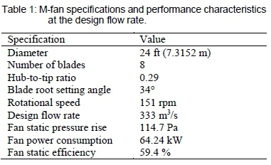
The fan under consideration in this study is the M-fan of Wilkinson et al. [5]. They evaluated the fan numerically using a three-dimensional periodic fan model with a zero tip clearance. The design specifications and performance characteristics of the fan at the design flow rate are listed in table 1.

 

 

Full-scale testing on ACC fans is often impractical due to their large physical size. The number of discharge configurations to test for the M-fan is also too extensive for scaled-down experiments. Computational fluid dynamics (CFD) was therefore used for the current investigation.

Prior to performing the simulations using the M-fan data, the CFD was validated against the experimental data of Clausen et al. [6] for swirling flow in a conical diffuser. The modelling strategies that provided the best results were then applied to the M-fan simulations.

Modelling the full-scale M-fan in detail would require enormous computational resources. The same holds for the blade passages of a downstream stator. Since the current study is only interested in the flow downstream of the M-fan, fixed outlet velocity profiles for the M-fan were used as inlet conditions for the computational domain. The fan was therefore not modelled. To simulate the effect of stator blades on the air stream, the extended actuator disc model (EADM) of Van der Spuy [7] was adopted. This model does not require detailed modelling of the blade passages and allows for a steady-state treatment of the flow through the stator. These simplifications substantially reduced the computational complexity of the flow problem.

The paper starts by demonstrating how pressure recovery affects the characteristics of an induced draught fan arrangement. Details of the numerical strategies and validation study follow. The pressure recoveries obtained with six different discharge configurations for the M-fan are then presented. Thereafter, the results of the configuration that had the highest pressure recovery were added to the M-fan characteristics to obtain the combined characteristics of the fan-diffuser unit. The paper ends with conclusions on the main findings.

 

2 Effect of Pressure Recovery on the Draught Equation of an Induced Draught ACC

The draught equation for an ACC is a mechanical energy relation that equates the mechanical energy supplied to the air by the axial flow fan to the energy dissipated through the ACC [8]. Pressure changes through the ACC are represented by a dimensionless pressure loss or gain coefficient, i.e.

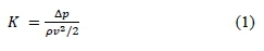
where ∆p represents the pressure loss or rise, p is the air density, and v is an average velocity based on a characteristic cross-sectional area.

The draught equation for the induced draught ACC shown in figure 1 is given by

 

 

 

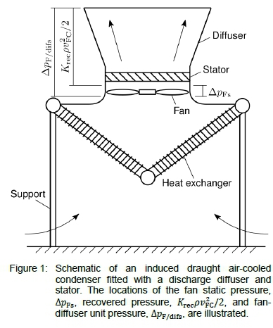
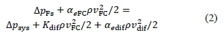
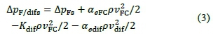
where ∆p_Fs denotes the fan static pressure rise, a_eFCthe kinetic energy flux factor at the discharge plane of the fan, and v_FC = V/A_FCis the mean axial velocity through the fan casing. The sum of the total pressure losses through the ACC, excluding that of the diffuser and discharge kinetic energy loss, is represented by Ap_sys. The excluded losses are given by the last two terms, where K_difis the total pressure loss coefficient of the diffuser and a_edif is the kinetic energy flux factor at the diffuser outlet. v_difis the mean velocity at the diffuser outlet.

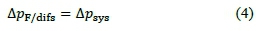
Since a_eFC, K_difand a_edifare generally unknown, Kröger [9] argued that it is useful to obtain the performance characteristics of the fan-diffuser unit. Four terms in equation (2) can then be replaced by

which simplifies the draught equation to

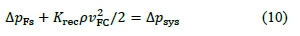
In order to distinguish between ∆p_Fs and ∆p_F/_difs, a pressure recovery coefficient, K_rec, is introduced. It accounts for both the kinetic energy at the fan outlet that is recovered within the discharge diffuser or stator as well as the frictional and local losses. The coefficient is defined as

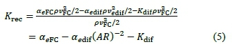
where AR = A_dif/A_FC is the area ratio of the diffuser. The kinetic energy flux factor is calculated by

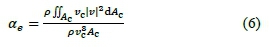
where v_cis the mean axial velocity through a cross-section of area A_c and |v| = . The kinetic energy flux factor at the fan outlet is thus equal to

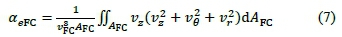
Equation (7) can be decomposed into components so that ^ae_FC = ^ae_FCz + ^ae_FC9 + ^ae_FCr. Near the design point of a free-vortex axial flow fan, the radial velocity is negligibly small so that a_eFCr~ 0. The axial component is given by

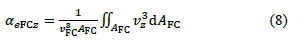
and the tangential component is given by

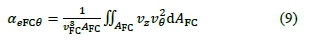
The minimum value for a_eFCz is equal to unity whereas the minimum value for a_eFC0 is zero.

Equations (7) to (9) together with equation (5) show how a diffuser or stator recovers pressure: If a stator can eliminate the swirl exiting the fan, then a_edif~ a_eFC - a_eFCe« a_eFCz. Note that a_eFC = 1.45, a_eFCe = 0.26 and a_eFCz = 1.20 for the M-fan at the design point. With a diffuser, a_edif and k_dif are both functions of the area ratio. The aim would thus be to find a diffuser with the largest possible area ratio which yields reasonably undistorted discharge velocity profiles (for a low a_edif-value) and a low total pressure loss, K_dif.

Substituting equation (5) into equation (2) produces the following form of the draught equation which can be used to determine the operating point of the ACC, i.e.

The theoretical maximum operating flow rate, V_max, would occur if K_rec = a_eFC. In this case, the available pressure would be equal to the fan total pressure rise, i.e. ∆p_Ft = ∆p_Fs + a_eFCpv²_FC/2. However, a_edif> 1 due to continuity, AR is limited by diffuser stall, and K_dif > 0 due to viscous and local losses. The available pressure will, therefore, lie somewhere between the extremes of the static and total pressures, as depicted in figure 2.

 

 

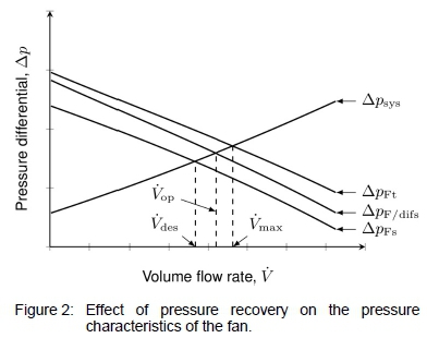
From figure 2 it can be seen that pressure recovery will shift the operating point to a higher volume flow rate, V_op, compared to the initial design flow rate, V_des. The increased airflow rate allows for higher heat removal rates in the ACC. Smaller overall plant structure sizes might, therefore, be possible due to pressure recovery. In addition, if it is assumed that the power characteristics of the fan remain unchanged after adding a diffuser or stator, the static efficiency of the fan system will increase. This assumption is not without merit as Terzis et al. [10] found that the power consumption of a small fan did not change after adding outlet guide vanes.

 

3 Numerical Modelling

The current investigation employed the open-source CFD code, OpenFOAM 5.0. It was used to solve the Reynolds-averaged Navier-Stokes equations for steady incompressible turbulent flows. Simulations that did not involve stator blade rows were computed using the simpleFoam solver.

Simulations that involved stator blades were solved using the EADM solver of Engelbrecht [11]. This solver was obtained by incorporating the EADM into OpenFOAM's buoyantBoussinesqSimpleFoam solver. The EADM is an axial flow fan model that was developed by Van der Spuy [7] to improve on the original actuator disc model (ADM) of Thiart and Von Backström [12]. These models make use of isolated aerofoil theory to calculate the force exerted by a fan blade on the air. The flow at the leading and trailing edges of the fan blade as well as the blade profile and orientation along the blade span are taken into account. Multiple researchers successfully employed these models to represent axial flow fans [13-16]. However, in this study, the EADM was used to model stationary stator blades downstream of an axial flow fan.

Pressure-velocity coupling was achieved using the SIMPLE algorithm. Gradient terms were discretised with the second-order central-differencing scheme. Bounded second-order linear-upwind and first-order upwind schemes were used for the advection of velocity and turbulence quantities, respectively. Laplacian terms were discretised using linear interpolation and the limited-corrected scheme with a stabilising coefficient of 0.33 for surface-normal gradients.

The pressure equation was solved using a geometric-algebraic multi-grid (GAMG) linear solver. The stabilised preconditioned bi-conjugate gradient (PBiCGStab) linear solver was employed for the velocity and turbulence equations. Pressure was under-relaxed by 0.2, velocity by 0.6 and turbulence variables by 0.7.

The kinematic viscosity and density of air at 20° were used in all simulations, i.e. v ~ 1.5 x 10^-5 and p ~ 1.2 kg/m³, respectively. Solutions were deemed converged after the static pressure at the inlet boundary had reached a constant value and the normalised residuals for all equations had reduced to at least 10^-5.

 

4 Numerical Validation

A representative test case with published experimental data was selected to validate the CFD. The modelling strategies that provided the best results were then applied to the M-fan simulations.

4.1 ERCOFTAC conical diffuser

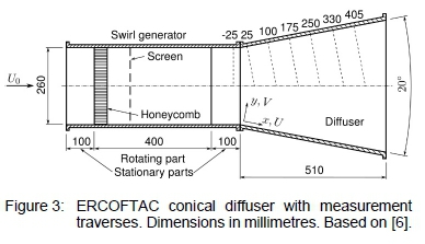
Clausen et al. [6] took detailed measurements of a swirling boundary layer developing in a conical diffuser of included angle 20° and area ratio 2.84, depicted in figure 3. This test case became known as the ERCOFTAC conical diffuser and has been the subject of multiple numerical studies [17-21]. The swirl generator produced an inlet swirl profile of a solid-body rotation and near-uniform axial velocity in the core region. The inlet swirl was sufficient to prevent boundary layer separation but insufficient to cause flow reversal at the centreline. The average inlet axial velocity was U₀ = 11.6 m/s and the inlet swirl number was W_max/U₀ = 0.59, where W_maxis the maximum circumferential velocity at the diffuser inlet. The diffuser discharged into the open atmosphere. Mean velocity and turbulent Reynolds stresses were measured in the diffuser along seven traverses normal to the wall. These traverses are illustrated by the dashed lines in figure 3.

 

 

4.2 Computational setup

The computational domain and boundary conditions are depicted in figure 4. The domain was inspired by that of Gyllenram and Nilsson [18]. However, they used an inlet extension to simulate the effect of the swirl generator, and an outlet extension to direct the flow out of the domain to improve numerical stability. Since experimental data are available at the inlet of the diffuser and numerical stability was not an issue, these inlet and outlet extensions were discarded. The geometry was wedge-shaped in the tangential direction and one cell thick. The wedge angle was five degrees, as recommended by the OpenFOAM user manual [22] for axisymmetric flow problems. The computational mesh comprised of hexahedral elements.

 

 

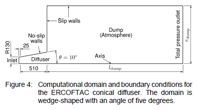
Velocity and turbulence kinetic energy profiles at the inlet (i.e., X = -25 mm) were interpolated from the experimental measurements of Clausen et al. [6]. The inlet pressure boundary condition was set to zero gradient. The diffuser wall was a no-slip boundary with a zero gradient pressure condition. The dump walls were slip walls with zero gradients for all remaining variables. A total pressure boundary condition of zero was specified at the outlet along with zero gradients for velocity and turbulence quantities. The axisymmetric planes were set to wedge boundaries, which are essentially cyclic boundaries.

4.3 Sensitivity studies

Various sensitivity studies were performed. These included the sensitivity to grid density, boundary distances, and inlet turbulence quantities. High- and low-Reynolds-number turbulence models were tested, and finally transient and three-dimensional effects were investigated.

The realisable k-e model of Shih et al. [23] with standard wall functions was used for the initial sensitivity studies. The turbulence dissipation rate at the inlet was computed with

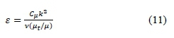
where C_μ = 0.09, v = 1.5 x 10^-5 and μ_t/μ = 14.5. The latter turbulent viscosity was adopted from Bonous [19].

4.3.1 Grid dependence

For the grid dependence study, the dump length, l_dump, and radius, r_dump, were fixed to ten diffuser inlet diameters and five diffuser outlet radii, respectively. Five grids with 13 040 to 208 640 nodes were tested for which the location of the first grid point in the diffuser ranged between y⁺ = 22 ~ 115 . The static pressure coefficient of the diffuser and flow profiles at the x = 330 mm traverse for the successively refined meshes were compared. With a grid of 104 565 nodes and y⁺~ 30, solutions were deemed to be grid-independent.

4.3.2 Boundary distance effects

The solutions were relatively insensitive to the dimensions of the discharge dump. Dump lengths of four to 14 diffuser inlet diameters were tested with a constant dump radius of five diffuser outlet radii. Dump radii ranging from one to seven diffuser outlet radii were tested with a constant dump length of ten diffuser inlet diameters. A dump with a length equal to eight diffuser inlet diameters and radius equal to five diffuser outlet radii produced boundary-distance independent solutions.

4.3.3 Inlet turbulence quantities

The sensitivity to inlet turbulence quantities was tested using different turbulent viscosities and length scales. The inlet turbulent dissipation rate for the realisable k-e model can be computed with equation (11) or

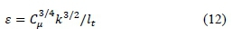
where l_tis the turbulent length scale. Turbulent viscosity ratios of 14.5 and 27.3 as well as a turbulent length scale of 3.2 mm were tested. These viscosity ratios were adopted from Bonous [19]. The length scale was used by Gyllenram and Nilsson [18] and is equal to the cell size of the honeycomb in the swirl generator. Solutions were affected by the specified inlet turbulent viscosity ratios and length scale. The results computed with the length scale of l_t= 3.2 mm compared the closest with the experimental measurements of Clausen et al. [6].

4.3.4 Turbulence models

Various turbulence models were tested. High-Reynolds-number models employed standard wall functions at no-slip boundaries. Liu [24] explains the implementation of these wall functions in OpenFOAM. The dimensionless distance from the wall was kept in the order of y⁺ ~ 30. The tested k-ε based models included the standard [25], realisable [23], renormalized group (RNG) [26], and quadratic [27] versions. The standard [28] and shear-stress transport (SST) [29] k-ω models were also tested. Two Reynolds-stress models (RSMs), namely the LRR [30] and SSG [31] models, were added to the investigation. The above models produced the streamwise velocity and turbulent kinetic energy profiles at the last measuring traverse (i.e., x = 405 mm) shown in figure 5. As in agreement with the findings of Dhiman et al. [20], the SST k-ω model performed very poorly.

For the low-Reynolds-number models, near-wall grid clustering allowed for integration through the viscous sublayer so that y⁺ ~ 1. Wall functions were thus avoided. At no-slip boundaries, the turbulence kinetic energy was explicitly set to zero. The k-e models that were tested included that of Launder and Sharma [32] as well as the cubic non-linear version of Lien et al. [33]. The turbulence dissipation rate, however, still required a wall function to describe the behaviour ε = 2vk/y²as y -> 0. The wall-integrated standard and SST k-ω models were also tested. Since the frequency ω tends to infinity at the wall, a large value (i.e., o = 10¹⁰ s^-1) was specified at the wall. Finally, the modified four-equation v'^2-f model of Lien and Kalitzin [34] with the limit of Davidson et al. [35] was included in the investigation. At the wall, v'²and ƒ were set to zero. Figure 6 contains the distributions at the last measuring traverse for these models. The SST k-o model again clearly performed the worst.

It is difficult to make a conclusive statement as to which of the tested turbulence models performed the best. Multiple studies demonstrated that k-e models with or without wall functions are incapable of resolving the flow in diffusers [3639]. Wall functions are generally not applicable in adverse pressure gradients [28], and damping functions lack a sound physical basis [40]. The more sophisticated four- and six-equation models do not show any clear advantage for this flow scenario. The wall-integrated k-o model was therefore selected: its results compare fairly well with the measurements and it does not require wall or damping functions.

4.3.5 Transient and three-dimensional effects

The final check was to determine whether the axisymmetric boundary condition and the steady-state assumption eliminated physical aspects of the problem. Both transient and steady-state simulates were performed on two-dimensional axisymmetric and three-dimensional meshes. Contrary to the findings of Dhiman et al. [20], the results of these four cases were essentially the same. Consequently, steady-state axisymmetric simulations were deemed sufficient.

 

5 M-Fan Discharge Configurations

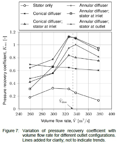
Diffusers, stator blade rows, or a combination of these can convert a portion of dynamic pressure into static pressure, i.e. recover pressure. Various outlet configurations were tested for the M-fan to find the configuration that provides the highest pressure recovery at design and off-design flow rates. The following discharge configurations were tested: a stator alone, conical and annular diffusers with and without stators at their inlets, and an annular diffuser with a stator at its outlet. Finally, the pressure recoveries of the best performing configuration were added to the characteristics of the M-fan to obtain the fan-diffuser characteristics.

5.1 Computational setup

The computational setup and solver settings were similar to those of the validation study. The wall-integrated k-ω turbulence model was used for all simulations with y⁺ ~ 1 at no-slip boundaries. Solutions that were deemed independent of the mesh density and the dimensions of the discharge dump were found for each of the different discharge configurations.

The inlet of the computational domain started at the outlet of the M-fan. The fan itself was thus not modelled. Fixed velocity and turbulence profiles at the fan outlet were used to specify the inlet boundary conditions. Circumferentially averaged outlet profiles for the M-fan at flow rates ranging from 260 to 380 m³/s were obtained from Wilkinson [41]. He measured these profiles from the hub to the tip of a periodic three-dimensional CFD model, approximately 0.1 m downstream of the fan blade trailing edge at the hub. Since Wilkinson [41] used the realisable k-e turbulence model, the turbulence dissipation rate had to be converted to turbulence frequency using ω = e/(ß*k), where ß^* = 0.09 [42].

5.2 Stator details

The stator blade rows were designed using the isolated aerofoil methodology outlined in Louw et al. [43]. The stator row at the outlet of the M-fan had nine blades and a mean chord length of 1.286 m. It was located at a half mean stator chord length downstream of the M-fan, as recommended by Wallis [4]. This stator was capable of removing all the swirl exiting the M-fan.

The discharge configuration with a stator row at the outlet of an annular diffuser had to have more stator blades and could only remove a portion of the swirl in order to obtain realistic chord lengths. The stator row had 13 blades with a chord length that varied between 1.29 m at the hub to 1.52 m at the tip. It could only remove 45 % of the swirl.

5.3 Method

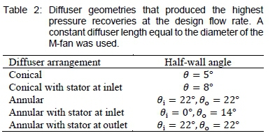
Similar to Walter et al. [3], it was decided to fix the diffuser length equal to the diameter of the fan. Parametric studies were performed at the design flow rate of the M-fan: The diffuser area ratio was changed by varying the opening angle of the diffuser. For configurations with conical diffusers, the half-wall angle (angle measured between the diffuser wall and axial direction) was varied within the range of 0° < 0 < 20° in increments of one degree. Various combinations of inner and outer half-wall angles were tested for the annular diffusers: The inner half-wall angle was varied in the range of 0° < 0_i< 30° in increments of two degrees;

a range of outer half-wall angles, 0_o, was tested for each one of these inner wall angles. Approximately 90 simulations were necessary to find the annular diffuser geometry that provides the highest pressure recovery.

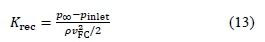
The recovered pressure was obtained by subtracting the area-weighted average of the inlet pressure, P_inlet, from the outlet pressure, p_∞. Subsequently, the pressure recovery coefficient was computed with

5.4 Results

5.4.1 Pressure recoveries for different discharge configurations

The diffuser geometries that produced the highest pressure recoveries at the design flow rate of the M-fan are summarised in table 2. After the best geometries were found for the design flow rate, they were tested at off-design flow rates. Figure 7 presents the results. Near the design flow rate, the annular diffusers with and without a stator at their inlets perform similarly. However, at lower off-design flow rates, the annular diffuser alone produces higher pressure recovery coefficients. This diffuser is thus recommended for the M-fan since it provides good pressure recoveries at both design and off-design flow rates.

 

 

 

 

5.4.2 Effect of pressure recovery on fan characteristics

Figure 2 illustrated how pressure recovery could shift the operating point to a higher volume flow rate than the initial design flow rate. The pressure recovery data for the recommended 22° equiangular annular diffuser were added to the characteristics of the M-fan to obtain the combined fan-diffuser characteristics. Figures 8 and 9 depict the fan-diffuser static pressure and static efficiency characteristics, respectively. A system curve of the form ∆p_sys = aV²that passes through the origin and the design point was included in figure 8. The static efficiencies were computed with N_Fs= ∆_pfsV/P_fand N_jF/difs= ∆_pF/áifsV/P_f, where P_fis the fan power consumption and ∆p_F/_difs = ∆p_Fs + K_recpv²_FC/2.

 

 

 

 

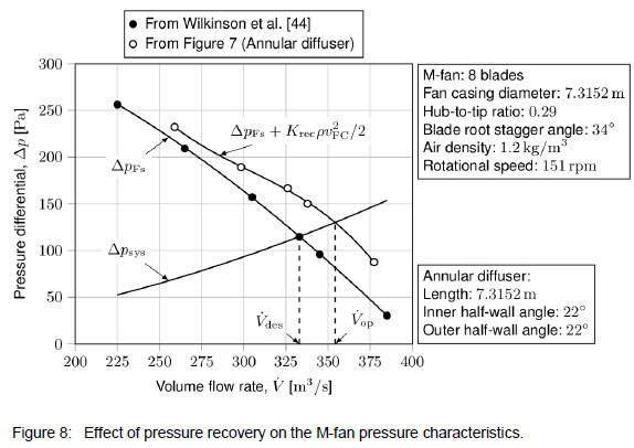
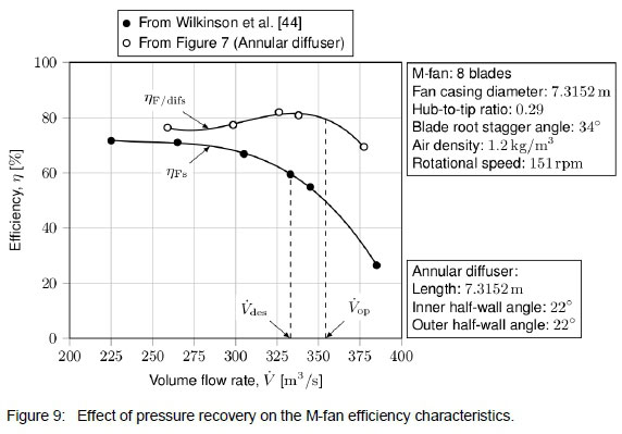
Pressure recovery raised the static pressure from 114.7 Pa at the initial design point to 130.0 Pa at the new operating point, i.e. a 13.3 % relative increase. The flow rate through the fan increased from 333.0 to 354.2 m³/s, i.e. a 6.3 % relative increase. The static efficiency at the new operating point is 79.4 %. This is 20.0 % (absolute) higher than the static efficiency of 59.4 % at the initial design point.

 

6 Conclusions

This paper outlined the theory of pressure recovery for an induced draught fan arrangement and provided pressure recovery data for various fan discharge configurations. A pressure recovery coefficient, K_rec, was introduced into the draught equation. It represents the pressure that is recovered within the discharge diffuser, stator, or diffuser-stator combination.

For numerical validation, CFD was used to simulate the swirling flow in the ERCOFTAC conical diffuser. Steady-state simulations on two-dimensional axisymmetric computational grids proved sufficient. Results were sensitive to the specified inlet turbulence quantities. Various high-Reynolds-number turbulence models with standard wall functions were tested as well as low-Reynolds-number models with integrated boundary layers. The results obtained with the wall-integrated k-ω model compared reasonably well with experimental measurements. The SST k-ω model performed poorly, with or without wall functions.

The validated CFD approach was then used to simulate six different discharge configurations for the M-fan in an induced draught arrangement. These included a downstream stator, conical and annular diffusers with or without stators at their inlets, and an annular diffuser with a stator at its outlet. An equiangular annular diffuser without a stator produced the highest pressure recovery coefficients over a range of flow rates. It had wall angles of 22° from the axial direction and a length equal to the diameter of the M-fan, i.e. 7.3152 m.

With a system curve of the form ∆p_sys = aV², the pressure recovery achieved with the equiangular diffuser increased the volume flow rate through the M-fan by 6.3 % (relative). The static efficiency at the new operating point was 79.4 %. This is 20.0 % (absolute) higher than the efficiency at the initial design point of the fan.

This study demonstrated that significant gains in fan performance are available through pressure recovery. However, the costs associated with pressure recovery installations have limited their application in practice. With the rising costs of energy, pressure recovery devices might become a valuable proposition for fan industries in the future.

 

References

[1] D. G. Kröger. Fan performance in air-cooled steam condensers. Heat Recovery Systems and CHP, 14(4):391-399, 1994.         [ Links ]

[2] J. Moore, R. Grimes, A. O'Donovan and E. Walsh. Design and testing of a novel air-cooled condenser for concentrated solar power plants. Energy Procedia, 49:1439-1449, 2014.         [ Links ]

[3] J. Walter, S. Caglar and M. Gabi. Investigation of the maximum static efficiency of axial fans. In International Conference of Fan Noise, Aerodynamics, Applications and Systems, Darmstadt, Germany, 2018.

[4] R. A. Wallis. Axial Flow Fans and Ducts. John Wiley & Sons, 1983.

[5] M. B. Wilkinson, S. J. Van der Spuy and T. W. Von Backström. The design of a large diameter axial flow fan for air-cooled heat exchanger applications. In ASME Turbo Expo 2017: Turbomachinery Technical Conference and Exposition, Charlotte, NC, USA, 2017.

[6] P. D. Clausen, S. G. Koh and D. H. Wood. Measurements of a swirling turbulent boundary layer developing in a conical diffuser. Experimental Thermal and Fluid Science, 6(1):39-48, 1993.         [ Links ]

[7] S. J. Van der Spuy. Perimeter Fan Performance in Forced Draught Air-cooled Steam Condensers. PhD Thesis, Department of Mechanical and Mechatronic Engineering, Stellenbosch University, 2011.         [ Links ]

[8] C. J. Meyer and D. G. Kröger. Plenum chamber flow losses in forced draught air-cooled heat exchangers. Applied Thermal Engineering, 18(9-10):875-893, 1998.         [ Links ]

[9] D. G. Kröger. Air-cooled heat exchangers and cooling towers: Thermal-flow performance evaluation and design. Department of Mechanical Engineering, Matieland, 1998.

[10] A. Terzis, I. Stylianou, A. I. Kalfas and P. Ott. Heat transfer and performance characteristics of axial cooling fans with downstream guide vanes. Journal of Thermal Science, 21(2):162-171, 2012.         [ Links ]

[11] R. A. Engelbrecht. Numerical Investigation of Fan Performance in a Forced Draft Air-cooled Condenser. PhD Thesis, Department of Mechanical and Mechatronic Engineering, Stellenbosch University, 2018.         [ Links ]

[12] G. D. Thiart and T. W. Von Backström. Numerical simulation of the flow field near an axial flow fan operating under distorted inflow conditions. Journal of Wind Engineering and Industrial Aerodynamics, 45(2):189-214, 1993.         [ Links ]

[13] C. J. Meyer and D. G. Kröger. Numerical simulation of the flow field in the vicinity of an axial flow fan. International Journal for Numerical Methods in Fluids, 36(8):947-969, 2001.         [ Links ]

[14] C. J. Meyer and D. G. Kröger. Numerical investigation of the effect of fan performance on forced draught air-cooled heat exchanger plenum chamber aerodynamic behaviour. Applied Thermal Engineering, 24(2-3):359-371, 2004.         [ Links ]

[15] J. R. Bredell, D. G. Kröger and G. D. Thiart. Numerical investigation of fan performance in a forced draft air-cooled steam condenser. Applied Thermal Engineering, 26(8-9):846-852, 2006.         [ Links ]

[16] M. B. Wilkinson, F. G. Louw, S. J. Van der Spuy and T. W. Von Backström. A comparison of actuator disc models for axial flow fans in large air-cooled heat exchangers. In ASME Turbo Expo 2016: Turbomachinery Technical Conference and Exposition, Seoul, South Korea, 2016.

[17] S. W. Armfield, N.-H. Cho and C. A. Fletcher. Prediction of turbulence quantities for swirling flow in conical diffusers. AIAA Journal, 28(3):453-460, 1990.         [ Links ]

[18] W. Gyllenram and H. Nilsson. Very large eddy simulation of draft tube flow. In 23^rd IAHR Symposium on Hydraulic Machinery and Systems, Yokohama, Japan, 2006.

[19] O. Bonous. Studies of the ERCOFTAC conical diffuser with OpenFOAM. Research Report 2008:05, Department of Applied Mechanics, Chalmers University of Technology, Göteborg, Sweden, 2008.

[20] S. Dhiman, H. Foroutan and S. Yavuzkurt. Simulation of flow through conical diffusers with and without inlet swirl using CFD. In Proceedings of ASME-JSME-KSME 2011 Joint Fluids Engineering Conference, Hamamatsu, Japan, 2011.

[21] C. S. From, E. Sauret, S. W. Armfield, S. C. Saha and Y. Gu. Turbulent dense gas flow characteristics in swirling conical diffuser. Computers & Fluids, 149:100-118, 2017.         [ Links ]

[22] C. J. Greenshields. OpenFOAM: User Guide. 5^th ed. OpenFOAM Foundation Ltd., 2017.

[23] T.-H. Shih, W. W. Liou, A. Shabbir, Z. Yang and J. Zhu. The new k-e eddy viscosity model for high Reynolds number turbulent flows. Computers & Fluids, 24(3):227-238, 1995.         [ Links ]

[24] F. Liu. A thorough description of how wall functions are implemented in OpenFOAM. In Proceedings of CFD with OpenSource Software, 2016.

[25] B. E. Launder and D. B. Spalding. The numerical computation of turbulent flows. Computer Methods in Applied Mechanics and Engineering, 3(2):269-289, 1974.         [ Links ]

[26] V. Yakhot, S. A. Orszag, S. Thangam, T. B. Gatski and C. G. Speziale. Development of turbulence models for shear flows by a double expansion technique. Physics of Fluids A: Fluid Dynamics, 4(7):1510-1520, 1992.         [ Links ]

[27] T.-H. Shih, J. Zhu and J. L. Lumley. A realizable Reynolds stress algebraic equation model. NASA Technical Memorandum 105993, NASA Lewis Research Center, Cleveland, OH, United States, 1993.

[28] D. C. Wilcox. Turbulence Modeling for CFD. 2^nd ed. DCW Industries, 1998.

[29] F. R. Menter. Two-equation eddy-viscosity turbulence models for engineering applications. AIAA Journal, 32(8):1598-1605, 1994.         [ Links ]

[30] B. E. Launder, G. J. Reece and W. Rodi. Progress in the development of a Reynolds-stress turbulence closure. Journal of Fluid Mechanics, 68(3):537-566, 1975.         [ Links ]

[31] C. G. Speziale, S. Sarkar and T. B. Gatski. Modelling the pressure-strain correlation of turbulence: An invariant dynamical systems approach. Journal of Fluid Mechanics, 227:245-272, 1991.         [ Links ]

[32] B. E. Launder and B. I. Sharma. Application of the energy-dissipation model of turbulence to the calculation of flow near a spinning disc. Letters in Heat and Mass Transfer, 1(2):131-137, 1974.         [ Links ]

[33] F. S. Lien, W. L. Chen and M. A. Leschziner. Low-Reynolds-number eddy-viscosity modelling based on non-linear stress-strain/vorticity relations. In W. Rodi and G. Bergeles, editors, Engineering Turbulence Modelling and Experiments, Elsevier Series in Thermal and Fluid Sciences, volume 3, pages 91-100. Elsevier, 1996.

[34] F.-S. Lien and G. Kalitzin. Computations of transonic flow with the v²-f turbulence model. International Journal of Heat and Fluid Flow, 22(1):53-61, 2001.         [ Links ]

[35] L. Davidson, P. V. Nielsen and A. Sveningsson. Modifications of the V2 model for computing the flow in a 3D wall jet. In Proceedings of the International Symposium on Turbulence, Heat and Mass Transfer, Antalya, Turkey, 12 - 17 October 2003.

[36] S. W. Armfield and C. A. Fletcher. Comparison of k-ε and algebraic Reynolds stress models for swirling diffuser flow. International Journal for Numerical Methods in Fluids, 9(8):987-1009, 1989.         [ Links ]

[37] Y. G. Lai, R. M. So and B. C. Hwang. Calculation of planar and conical diffuser flows. AIAA Journal, 27(5):542-548, 1989.         [ Links ]

[38] G. Iaccarino. Predictions of a turbulent separated flow using commercial CFD codes. Journal of Fluids Engineering, 123(4):819-828, 2001.         [ Links ]

[39] S. M. El-Behery and M. H. Hamed. A comparative study of turbulence models performance for separating flow in a planar asymmetric diffuser. Computers & Fluids, 44(1):248-257, 2011.         [ Links ]

[40] V. C. Patel, W. Rodi and G. Scheuerer. Turbulence models for near-wall and low Reynolds number flows: A review. AIAA Journal, 23(9):1308-1319, 1985.         [ Links ]

[41] M. B. Wilkinson. The Design of an Axial Flow Fan for Air-cooled Heat Exchanger Applications. Master's Thesis, Department of Mechanical and Mechatronic Engineering, Stellenbosch University, 2017.         [ Links ]

[42] D. C. Wilcox. Reassessment of the scale-determining equation for advanced turbulence models. AIAA Journal, 26(11):1299-1310, 1988.

[43] F. G. Louw, P. R. P. Bruneau, T. W. Von Backström and S. J. Van der Spuy. The design of an axial flow fan for application in large air-cooled heat exchangers. In ASME Turbo Expo 2012: Turbomachinery Technical Conference and Exposition, Copenhagen, Denmark, 2012.

[44] M. B. Wilkinson, S. J. Van der Spuy and T. W. Von Backström. Performance Testing of an Axial Flow Fan Designed for Air-Cooled Heat Exchanger Applications. In ASME Turbo Expo 2018: Turbomachinery Technical Conference and Exposition, Oslo, Norway, 2018.

 

 

Received 9 December 2019
Revised form 24 June 2020
Accepted 24 June 2020