Characterisation of submerged arc welding process using infrared imaging technique

 

 

M.C. Zondi^I; Y. Tekane^II; E. Magidimisha^III; E. Wium^IV; A. Gopal^V; C. Bemont^VI

^IDiscipline of Mechanical Engineering. University of KwaZulu Natal, Durban, South Africa. zondi@outlook.com
^IICSIR DPSS, Landward Sciences, yanga.tekane@gmail.com
^IIICSIR DPSS, Optronics, EMagidimisha@csir.co.za
^IVCSIR DPSS, Landward Sciences, EWium@csir.co.za
^VCSIR DPSS, Landward Sciences, AGopal@csir.co.za
^VIDiscipline of Mechanical Engineering. University of KwaZulu Natal, Durban, South Africa. bemontc@ukzn.ac.za

 

 

---

ABSTRACT

Infrared (IR) thermography is a technique used to measure temperature distribution of heat generation in manufacturing processes such as welding. IR thermography is a non-destructive and non-contact method, which makes it favoured for the arc welding process where interference with the welding process must be avoided. In this study, IR thermography is used to record the temperature history during the submerged arc welding (SA W) process experiment; and to validate the numerical model developed to simulate the said SAW process of a multi-pass circumferential weld on pressure vessel steel. The Flir Short Wave Infrared Radiometer (FSIR) is used during SAW experiments with the ESAB welding unit. The weld pool and the surrounding area are continuously monitored and their temperature recorded using a thermal camera. The recorded temperatures are plotted against time on Temperature-Time curves to reveal the temperature profiles of each welding cycle. Comparison of the resultant temperature profiles with those of the numerical model show good agreement. It is therefore concluded that temperature measurement through thermal imaging is a suitable method to characterize the temperature history of the SAW multi-pass circumferential weld, as well as to effectively validate the numerical model developed to simulate the said welding process.

Additional keywords: Infrared thermography, temperature distribution, submerged arc welding, welding parameters, numerical analysis

---

 

 

Nomenclature

SAW Submerged Arc Welding

TIG Tungsten Inert Gas

GTAW Gas Tungsten Arc Welding

MIG Metal Inert Gas

FR Wire Feed Rate

CA Constant Amperage

CW Constant Wire

HAZ Heat Affected Zone

IR Infrared

SWIR Short Wave Infrared

FSIR Flir Short Wave Infrared Radiometer

FEA Finite Element Analysis

CFD Computational Fluid Dynamics

3D Three Dimensional

ANN Artificial Neural Networks

Roman

d Outside Diameter of the Pipe

S Rotational Speed

T₀ Ambient Temperature

Τ Surface Temperature of the Weld Pool

t Time

Greek

є Emissivity

σ Stefan-Boltzmann Constant

h Convection Coefficient

 

1 Introduction

Infrared (IR) thermography is getting more and more popular in arc welding applications. The ability to continuously record welding temperatures in the weld pool and the surrounding surface without any physical interference (i.e. non-contact process) of the actual welding process makes IR thermography the preferred measurement method over point sensors such as thermocouples. IR thermography produces continuous temperature distribution profiles of the weld area of interest through recordings using a thermal camera. Application of IR thermography in metal welding includes real-time monitoring of the weld pool, weld defect identification, weld geometry determination, auto-correction of welding parameters (when used with soft computing), and many more. IR thermography is also used for on-line monitoring and control of welding parameters in automation processes using intelligent methodologies. The utility of online defect identification is in that it saves cost of post weld defect identification, which inevitably leads to rejection or rework. The basis for using thermal sensors for identification of defects and/or monitoring of weld geometry is in that the surface temperature distribution during welding should ideally show a regular and repeatable pattern; and any deviation can be identified through perturbations or variations in temperature profiles.

The advantage of the IR thermal imaging method over other sensors such as thermocouples is that it provides continuous measurement over a larger area of interest. The other advantage of IR thermography is its ability to monitor several parameters simultaneously, thereby eliminating the need for multisensory systems. Thermal imaging is also capable of handling rapid welding speeds and short thermal response times associated with arc welding. The thermal imaging technique is not without shortcomings. One of the well-known drawbacks of thermal imaging is that the accuracy of the IR thermal camera is a function of material emissivity, which in turn is affected by the surface condition of the material.

This paper presents the temperature history of the welding cycle in the nozzle-to-shell circumferential weld of the pressure vessel using IR thermography. The objective of the study is to show the effectiveness of IR imaging in accurately mapping out temperature histories of the Submerged Arc Welding (SAW) process, as well as using IR thermography as means of validating the numerical model. The next section presents the literature survey of similar studies; section three discusses the numerical model, whereas the fourth section presents the experimental work. Results are discussed in section five, and the conclusion is given in the last section.

 

2 Literature Review

Wikle et al. [1] develop a rugged, low cost, point infrared sensor that is used to monitor and control the welding process. Heat transfer analysis is performed to study the effects of the plate surface temperatures to the weld geometry, occurring during the welding process. This is correlated to actual measurements from the IR sensor monitoring changes in the plate surface temperature during the welding process. The weld bead penetration depth is measured and compared to the prediction of the heat transfer analysis. Infrared thermography is used to monitor and control weld geometry during the Tungsten Inert Gas (TIG) welding process of stainless steel 316LN plates [2]. The produced thermal images are analysed to determine temperature distribution patterns that give effect to weld geometry and that give indication of the nature of weld defects in the weld pool. The developed technique can be used as a basis for the adaptive/intelligent weld methodology.

A study by [3] highlights the application of thermal imaging sensors for detection of defects such as lack of penetration and estimation of depth of penetration during TIG welding. Results show that IR imaging technique can adequately detect lack of penetration and depth of penetration online. Thermal imaging and visual band camera are the main vision sensors used during on-line monitoring. A system based on the application of one thermal vision camera and two charged-coupled device (CCD) cameras for assessment of a welding process and welded joints is presented in [4]. Literature [5] proposes a method for calibration, tracing and accreditation of thermal imagers through the implementation of best international measurement practices. The study by [6] uses thermography to determine weld bead geometry and weld defects in real-time during the Gas Tungsten Arc Welding (GTAW) process of stainless steel. The weld bead geometry results obtained using line-scan analysis of the IR thermal profiles is successfully correlated to the values obtained through experimentation, with the correlation coefficient of 0.8. The defects identified through thermal images are verified using X-Ray radiography.

In their study to identify weld defects of the TIG welding process through thermal imaging, [7] show that the weld defects identified through thermography compares well with those discovered through X-Ray method. One of the main challenges experienced through this study is the difficulty in tracking the correct thermal history of the weld region, given that the IR camera targeted a moving region of interest. One way of mitigating the impact of such limitation is to increase the area of interest to include more than just the weld pool.

IR thermography is used to perform seam tracking, penetration control, bead width control, and cooling rate control to ensure acceptable weld quality [8]. Artificial Neural Networks (ANNs) are used in conjunction with thermal imaging to predict weld bead geometry. The ANN model is validated using experimentally measured values and the correlation coefficient of 0.99 is attained. Bai et al. [9] introduce a new approach of calibrating welding parameters in the weld-based additive manufacturing process using IR imaging and inverse analysis. In-depth analysis of thermal images vis-à-vis the simulation results produces comparable parameters such as mean layer temperature and cooling rate, which are used in cost functions. Comparison of predicted and measured values show an error in temperature history less than 30 °C. The study concludes that temperature measurements using IR imaging is far better than thermocouples for weld-based additive manufacturing applications.

IR thermography is used to experimentally validate the finite element analysis (FEA) model for a Submerged Arc Welding (SAW) joint on a steel plate [10]. The authors observe that the insulating granular flux present in the SAW process makes thermal imaging difficult. Some researchers have suggested the use of flux removal methods such as vacuuming immediately behind the weld-pool. The authors in [10] manufactured a special U-shaped piece to keep the flux away from the region of interest so that temperature measurements, which took place away from the fusion zone, could be done efficiently. The temperature values predicted using numerical methods are found to be in reasonable agreement with the experimental results. The accuracy of the finite element model is found to be acceptable for the identified parameters, with R-square values ranging between 0.96 and 0.99. Numerical methods are used to model the metal surfacing process using the metal inert gas (MIG) welding technique. Thermography is used to validate the numerical results [11]. The thermal camera is used to determine temperature distribution through recording temperature at various points of the surface. The images from numerical analysis are compared with those produced through thermal imaging, and they appear to be very similar. An application of infrared imaging technique in a HighPower Fibre Laser welding process of stainless steel 304L to monitor the weld pool width to automatically control the welding process can be seen in [12]. Comparison of predicted and measured values show good correlation with a maximum error of 0.0994. A proposed remote welding process based on a methodology that combines image processing with soft computing to estimate bead geometry is presented by [13]. The real-time bead geometry monitoring allows for on-line parametric adjustments during the Tungsten Inert Gas (TIG) welding process of stainless steel.

 

3 Experimental Procedures

The experimental setup consists of the ESAB SAW machine and the Short-Wave Infrared (SWIR) camera as shown in figure 1. The SAW machine has two major components, viz. the wire feeder and the turntable. The turntable is a requirement for conducting circumferential welds, wherein the turntable speed is converted to linear welding speed. The consumable welding electrode is fed into the weld-pool through the wire feeder during the welding process. The wire feed rate (FR) is controlled by the ESAB controller as can be seen in figures 1 and 2.

 

 

 

 

 

 

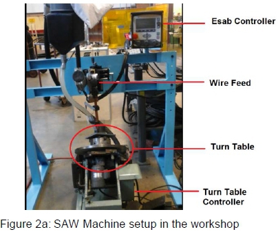
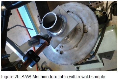
The controller used is commissioned with the SAW machine and operates in one of two modes; the user can either select a constant amperage (CA) mode or a constant wire (CW) feed rate mode. In CA mode, the operator selects the required current, and the FR is automatically chosen by the controller, such that the operator has no control of the latter. In CW mode, the similar setup occurs, but this time the operator selects the FR and the current is automatically set by the controller. In the present study all the test specimens were prepared in CA mode. Figure 2(a) illustrates the setup for experiments as was prepared in the mechanical workshop. Figure 2(b) is a magnification of the turntable from figure 2(a).

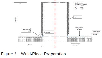
The experimental design focuses on capturing the temperature history and distribution across the overall structure of the weld sample. The advantage of the IR thermal imaging process over pointed sensor-based methods such as thermo-couples is that the former can record the entire area of interest at a single instance, given its broad coverage. This effectively means that data are recorded for an infinite number of points of interest; and during data analysis such data can be retrieved from the image file for each point chosen. On the other hand, pointed sensors can only record data for one point at a time, and data analysis is limited to such a point only. The weld-piece consists of a 5 mm wall thickness steel pipe of 80 mm bore welded onto a 10 mm steel plate using a full penetration multi-pass weld as shown in figure 3. The illustration shown in figure 3 is typically the weld joint used for joining nozzles onto a cylindrical pressure vessel shell as prescribed in the appropriate design codes.

 

 

It was discussed above that the granular flux in SAW can present a challenge during IR thermography temperature measurements given its tendency to insulate the surface. In the present study, the Metal Inert Gas (MIG) welding process was used with the same heat input and welding parameters for the reference test specimen. This allowed the researchers to establish the temperature of the weld pool without the effect of insulation. It should be noted, however that, as long as the measurements are taken away from the weld-pool, and in the area with no granular flux insulation, then the above is not necessary; and that is why the latter approach was adopted for the purposes of validating the numerical model as discussed in section 4 below.

The pipe material is ASTM A106 and the plate is ASTM A516, chosen for practical purposes since these materials are typically used for pressurized system applications. A hole of the same size as the internal diameter of the pipe was drilled through the plate to position the pipe in the same way that the nozzle would be positioned on the pressure vessel. Low hydrogen high strength Spool Arc 18-F7A6-EM12K electrodes were used. A three-pass full penetration weld was then performed using the SAW process.

Temperature measurements were carried out using the Flir Ultra-High Resolution Thermal Camera (FLIR X6550SC) with the frame rate of 125Hz (at 640x512 IR resolution pixels) and +/-1°C accuracy. During measurement, the FSIR radiometer was placed at a focus range of 3m as shown in figure 1. Power to the FSIR was supplied via the standard 220 V, 50 Hz, single phase municipal supply and the FSIR was connected to the controller (PC) using the original equipment manufacturer (OEM) supplied camera link cable. The FSIR was left for five minutes to cool down before operation. This was done so that the camera could acclimatise to the ambient temperature of the laboratory. The Flir RerearchIR version 3.3 software was accessed on the controller and the configuration setup which matched the temperature of the scene was selected. This included the sensitivity parameters i.e. integration time and the neutral density filter. Before measurement could begin, a non-uniformity correction was performed to compensate for the variations in camera operating conditions and to improve image quality. The measurements were conducted in a closed environment and within a short time in order to minimize the impact of path radiance and atmospheric effects, which were consequently considered negligible. In addition, the SAW welding process is insulated by a layer of granular fusible flux which protects it from atmospheric attenuation.

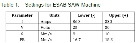
The SAW parameters chosen for the present study have been shown to demonstrate consistent and significant effect on the weld geometry, heat affected zone (HAZ) size, mechanical properties and residual stress [14]. Chosen parameters include welding current (I), arc voltage (V), travel speed (S) and wire-feed rate (FR). Each parameter has upper (+) and lower (-) limit chosen according to their safe operational ranges (see table 1). The range of values was chosen using guidelines from SAW machine operator's manual and practical welding experience. When choosing the operational range for SAW parameters, care should be taken to only include parametric combinations that will not result in burn-through or lack of penetration.

 

 

Seven weld specimens were prepared using the welding parameters mentioned in table 2. Each specimen was given a unique number (sample #) in order to easily track it as it underwent various evaluation processes.

 

 

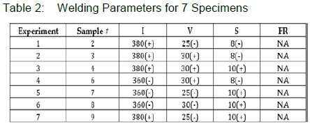
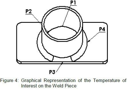
Table 3 gives the location of the respective recording points of the temperatures of interest on the sample, which were later used to plot the temperature profiles for the welded samples.

 

 

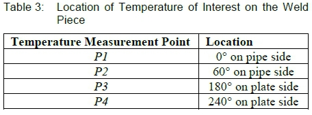
The recording points for the temperatures of interest given in table 3 are shown graphically in figure 4. It must be noted that P1 and P2 are measured from the inside of the pipe (weld root), whereas P3 and P4 are measured from the outside at weld-toe of the plate side.

 

 

4 Numerical Model

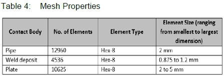
A three-dimensional (3D) model was created in MSC Marc to perform a coupled thermal-structural analysis. The computational model, shown figure 5, consists of 28121 eight-nodded hexagonal (hex) elements with an average mesh resolution of approximately 2mm. The mesh is more refined in the area of the weld, as shown in figure 5. The properties of the mesh are summarised in table 4. The plate, weld deposit and pipe were modelled as three separate bodies with contact specified between the bodies on the relevant surfaces to prevent penetration. The welding finite element analysis was performed as a coupled thermal-structural analysis.

 

 

 

 

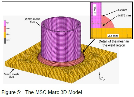
This is a non-linear analysis due to the non-linearity of the material model (i.e. elastic-plastic material). Beyond a certain point (yielding), the constitutive relation between stress and strain is not linear. The governing equation of the thermal analysis is conservation of energy which is used to solve for energy. The governing equations of the structural analysis are the equilibrium equations, constitutive relations and the compatibility equations to solve for the displacement, strain and stress fields. MSC Marc uses a staggered solution procedure in the coupled analysis; the heat transfer analysis is first performed, then the stress analysis. The model was created based on the MSC Marc example problem in [16].

Theory and additional background information on the solver is given in [17].

4.1 Model Assumptions

The following modeling assumptions were adopted for the thermal-structural model:

i. The pipe, plate and weld material have the same material properties and have been modelled as an elastic-plastic isotropic material with temperature dependent properties. Plasticity is governed by the Von Mises yielding function, associated flow rule and linear, isotropic work-hardening.

ii. Viscous material behaviour at high temperatures is neglected.

iii. Initial stresses and strains are ignored.

iv. Initial temperatures are taken as 29 °C.

v. Natural heat loss due to convection and radiation only. Conduction heat loss (i.e. to the turn table) is negligible. Heat loss coefficients remain constant.

vi. Welding efficiency of 85%.

vii. Simplified pipe geometry (the root gap between the pipe and the plate and the chamfer on the pipe as illustrated in figure 3 can be neglected).

viii. Simplified weld bead geometry.

ix. Simplified heat source model, as proposed by Goldak in [18].

x. The effect of annealing is not considered.

A convection and radiation heat loss boundary condition was applied to all the exposed surfaces of the sample, including the elements of the weld as soon as they are deposited. The heat transfer coefficient is taken as 15 W/m²K with an ambient temperature of 29 °C and emissivity of 0.625. Solid-liquid transformation is accounted for by specifying a latent heat of fusion of 270 kJ/kg with a solidus temperature of 1481 °C and liquidus temperature of 1510 °C.

4.2 Material Model

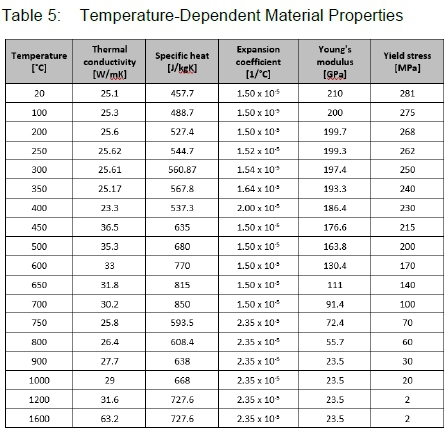
The steel was modelled as an elastic-plastic material with isotropic hardening, as proposed in [19]. The material properties of steel were taken from [20]. The temperature-dependent material properties are given in table 5. Young's modulus is taken as 210 GPa at 20°C and is varied with temperature, and the initial yield strength is 281 MPa and is varied with temperature. The specific loading/machining that the material has undergone has not been accounted for; yield strength values from [20] have been used. Specific heat capacity, thermal conductivity and thermal expansion coefficient and are also temperature dependent and the initial values at 20 °C are set to 457.7 J/kgK, 25.1 W/mK and 15x10^-6 1/°C respectively. Based on recommendations from [21], thermal conductivity was doubled for temperatures above the melting temperature (1400 °C). Poisson's ratio remains constant at 0.3. Changes in density are not specified, however an initial density of 7780 kg/m3 is specified and changes in density are automatically calculated by the solver as the volume changes with temperature.

 

 

5 Results

5.1 Experimental Results

The temperature versus time relationship was monitored during the welding experiments, and the presented results in this section focus on the two parameters. The expected time to complete a half perimeter revolution from P1 to P3 is 45n/S seconds as shown in equation 2, using the measured welding specimen diameter in equation 1. The time for Specimen 2 to do half revolution from P1 to P3 is shown in equation 2, where 'S' is the rotational speed indicated in table 2.

The measuring error is approximated by comparing the calculated time using equation 2 with the time measured from the IR thermal camera. Equation 3 is then used to calculate the error, and the results are tabulated in table 6. Note that inter-pass temperature refers to the time between weld passes. The IR camera records continuously and hence inter-pass time between first and second passes can be determined by obtaining the difference between the time at which the first weld pass ends and the time at which the second weld pass begins.

 

 

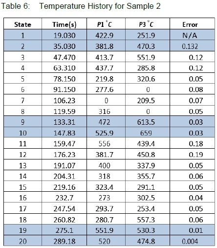
It is observed from table 6 that the measuring error is relatively larger in the beginning of the measurements as the thermal footprint of the specimen is much lower in the beginning of the welding process. The result of the low initial thermal footprint is that the marker cannot be viewed clearly at the beginning of the welding cycle. As the weld specimen temperature increases, the error decreases thereby increasing the accuracy of agreement between the calculated and the measured temperature values. The IR camera is calibrated to measure temperature from 200 °C up to 1700 °C and all values below 200 °C are therefore reflected as zero.

Figures 6 to 9 show experimental results for measuring temperatures for a three-pass weld performed in sample 2. As mentioned above, when starting the welding process (figure 6), marker is not clearly visible and the marker position can be approximated by adding theoretical 45n/S seconds from previously known marker time. Further to the times recorded by the IR camera and those calculated using equation 2, the stop watch was also used to manually record times from the beginning of each weld pass until the end.

 

 

 

 

 

 

 

 

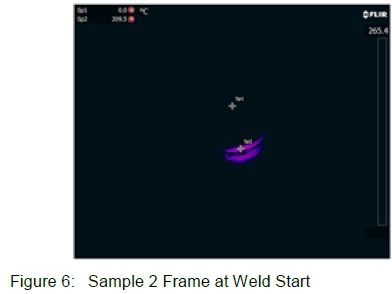
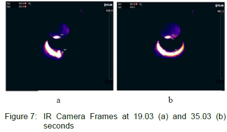
The frames from the IR camera clearly show the thermal footprint of the specimen during welding. Figure 6 shows the time immediately after the start of the welding process for the first pass. The specimen is still cold and hence the relatively small thermal footprint. Progress in the welding process can be seen in figure 7, which shows the temperatures for states 1 and 2 in table 6. State 1 represents approximately half of the first revolution of the first weld pass; whereas state 2 represents the end of the full revolution for the first weld pass. The incremental growth of the thermal footprint from figures 7(a) to 7(b) is clearly visible in the presented frames.

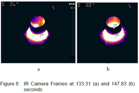
Since the experiment comprises a three-pass weld, two inter-pass temperatures are measured on two states. The first inter-pass time occurs from state 3 to state 8. In other words, the temperature in state 8 is the last recorded temperature before commencement of the second pass. Figure 8 illustrates the temperature footprint of states 9 and 10. The improvement in the overall visibility of the thermal image is indicative of the increased overall temperature of the specimen during the execution of the second weld pass.

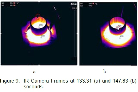
The third and final weld pass is represented in the frame in figure 9. The thermal image presented in this figure is the most clear of all the images, and the accuracy is the highest given the low error against the temperature values of states 19 and 20 in table 6. The marker is clearly visible in figure 9, and a circle is drawn around it to indicate its location. The reference marker is used to locate the specimen as it rotates relative to the position of Sp1 (P1) and Sp2 (P3).

Note that only six states from table 6 were chosen to demonstrate the illustration of the frames, and hence not all frames were presented in this write-up. The chosen states in table 6 have been highlighted for ease of reference.

5.2 Numerical Results

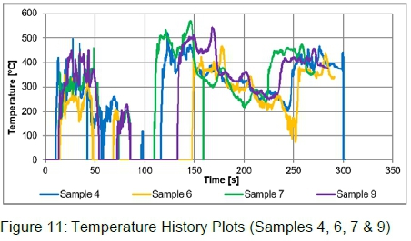
The numerical model was validated using temperature measurements obtained as illustrated in figure 10. The region of interest is a 5x5 pixel grid. The measurement region is located on the outside of the pipe, 6 mm above the weld and 180° from the arc. The average temperature of the region is plotted. The standard deviation was also monitored and was observed to be relatively insignificant. Four samples were analysed in the numerical model, namely 4, 6, 7 and 9.

 

 

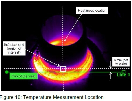
Figure 11 presents the temperature history plot of a fixed region on the pipe for each of the 4 samples. Temperatures are taken from the SWIR Camera system in the location presented in figure 10 for each specimen.

 

 

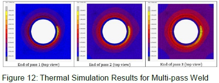
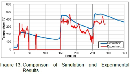
The typical simulation results for each of the three passes are illustrated in figure 12. Figure 13 presents the comparison in temperature history plots of Sample 6 between experimental and numerical analysis results.

 

 

 

 

6 Discussion

Figure 14 shows the temperature history plots of P1 and P3 in sample 2. The values used in generating the Temperature vs. Time graphs were taken from table 6. A close look at P1 graph shows that at 19 seconds (which is approximately half a revolution), the temperature is already above 400 °C, which is evident of the fact that the welding torch has already passed through the measuring point. This is in line with the IR image frames presented in figure 7.

 

 

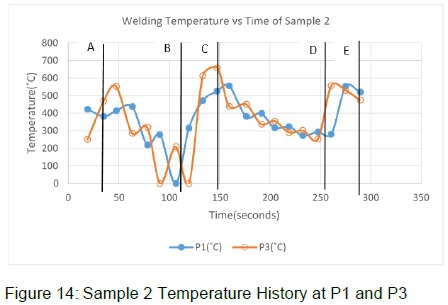
The point A represents the completion of the first weld pass, i.e. one revolution. Point B represents the commencement of the second weld pass. The segment AB therefore is the inter-pass time between the two passes. Given that there is no welding during the inter-pass time, it is expected that the weld will cool slowly under room temperature to lower temperatures. The profile of figure 14 however shows that the temperature at P1 increases slightly before falling every time. This can be accredited to the error between the calculated value (i.e. when the marker is not clearly visible), and the measured value (which is recorded by the camera). As explained above, the camera is calibrated between 200 and 1700 °C, and hence values outside this range are not detectable. The segment BC represents the duration for the second weld pass. It can be seen that higher peak temperatures are achieved during the second pass, and this is due to the temperature differences at inter-pass temperature (i.e. when the second pass begins) compared to room temperature (i.e. when the first pass begins). Similarly, the slope of the BC segment is less than that of the AB segment, signifying the lower cooling rate due to smaller temperature gradients of the latter.

The general profile of the graphs in figure 14 is indicative of the temperature distribution in a welding process observed in similar studies [14]. It can be seen that the peak temperatures recorded in P3 curve are higher than those observed in the P1 curve. This could be due to the positioning of the respective measurement points. P3 is located at the weld-toe on the plate side, while P1 is located at the root at point (0,0). The thermal footprints produced by the thermal camera images (figures 6 to 9) show that overall temperature of the specimen increases as more weld passes are added. This is because the accumulated heat input increases with the increase in weld passes. The finite element results shown in figure 12 are in agreement with the IR thermal images in that they also clearly show an increase in thermal footprint of the specimen as the number of weld passes increases.

The welding process is not perfectly smooth; therefore the temperature measurements also do not produce a smooth curve, as shown in figure 11. Chipping of the welding slag during the experiment also caused sharp peaks in the temperature readings (evident in figure 11). The comparison of simulation and experimental resultant temperature histories is shown in figure 13. The simulation results produce a smoother curve than the IR thermal camera, however the profile of the two curves is comparatively similar. The correlation between the two sets of results is therefore considered to be fair. The trends and the rate of cooling (gradient of the slope) correspond. The minor differences in the results can be accredited to the following reasons:

• The simulated welding process is a perfectly idealised process and external, uncontrollable factors are not taken into account. This refers to reflections from surrounding surfaces, the presence other heat sources, oversaturation of the detector, uncertainties in the measurements and errors in camera calibration.

• Other differences between reality and the simulated environment, such as the actual welding efficiency, convection heat loss coefficient, ambient temperature and the exact volume of the weld.

• Errors/limitations in the detector

• Material properties used were taken from literature

 

7 Conclusion

IR thermography has been shown to have advantages over pointed sensor techniques such as thermocouples. Such advantages include the following [15]:

i. It is a non-contact technology such that the devices used are not in contact with heat source. This allows very high temperatures within hazardous or dangerous environments to be measured safely.

ii. The 2D measurements make it possible to compare the regions of the area of interest.

iii. Real-time measurements allow high-speed scanning of stationary targets, temperature recording from fast-moving targets, and measuring from rapidly changing thermal patterns.

iv. IR thermography has no harmful substances (such as X-Rays) and can therefore be safely used for prolonged periods in a vast array of environments

v. The non-invasive nature means IR thermography does not physically affect the target in any way.

Thermal imagery characteristics of the SAW process, including temperatures distribution, inter-pass time, and cooling period have been clearly demonstrated in the present study. The readings taken from P1 and P3 and plotted in figures 6 to 9 are easily verifiable against figure 12, which visibly illustrates the change in thermal footprint of the specimens as more weld passes are deposited. Thermal imaging provides continuous measurement of temperatures, thereby allowing the Temperature-Time graphs to be plotted incorporating the cooling periods during welding cycles. This allows for better understanding of thermal behaviour of the weld pool during welding cycles. Furthermore, continuous temperature measurements also provide more accurate means to calibrate simulation models using recorded experimental temperatures.

The comparison between numerical results and experimental results shows good agreement, thereby indicating suitability of IR imaging as a technique to validate numerical models. The spikes in the experimental results can be accredited to the manual removal of slag through chipping. The slopes of the two graphs (simulation and experimental) are however comparable. The interpass temperature affects cooling rate, as has been shown in the varying slopes of the different weld passes. The cooling rates are affected by temperature gradients, which in turn result from accumulated heat input. Some of the challenges experienced during experimentation include the proper calibration of the thermal camera within the required temperature thresholds, the positioning of the camera vis-a-vis the rotating weld-piece for optimal temperature recordings, and the insulating effect of the flux in SAW the process.

IR thermography has been successfully utilised to characterise the SAW welding process and validate the numerical model. The produced SAW numerical model, having been calibrated and validated through experimental procedures, can be used for analysis of the nozzle-shell circumferential weld joint in cylindrical carbon steel pressure vessels.

 

Acknowledgements

The authors would like to thank the Council of Scientific and Industrial Research (CSIR) for allowing the use of its laboratory facilities in Pretoria, and for assisting with experimental work.

 

References

1. Wikle HC, Kottilingam S, Zee RH and Chin BA, Infrared Sensing Techniques for Penetration Depth Control of the Submerged Arc Welding Process, Journal of Materials Processing Technology, 113(1), 228-233, 2001.         [ Links ]

2. Menaka M, Vasudevan M, Venkatraman B and Raj B, Estimating Bead Width and Depth of Penetration During Welding by Infrared Thermal Imaging, Insight-Non Destructive Testing and Condition Monitoring, 47(9), 564-568, 2005.         [ Links ]

3. Venkatraman B, Menaka M, Vasudevan M and Raj B, Thermography for Online Detection of Incomplete Penetration and Penetration Depth Estimation. Proceedings of the 12^th Asia Pacific Conference on NDT5, 6 November, Auckland New Zealand, 2006.

4. Bzymek A, Czuprynski A, Fidali M, Jamrozik W and Timofiejczuk A, Analysis of Images Recorded During Welding Processes, Proceedings of 9^th QIRT Conference, July, 2008.

5. Machin G, Simpson R and Broussely M, Calibration and Validation of Thermal Imagers, Quantitative InfraRed Thermography Journal, 6(2), 133-147, 2008.         [ Links ]

6. Vasudevan M, Chandrasekhar N, Maduraimuthu V, Bhaduri AK and Raj B, Real-time Monitoring of Weld Pool During GTAW Using Infrared Thermography and Analysis of Infrared Thermal Images. Welding in the World, 55(7-8), 83-89, 2011.         [ Links ]

7. Sreedhar U, Krishnamurthy CV, Balasubramaniam K, Raghupathy VD and Ravisankar S, Automatic Defect Identification Using Thermal Image Analysis for Online Weld Quality Monitoring, Journal of Materials Processing Technology, 212(7), 1557-1566, 2012.         [ Links ]

8. Chokkalingham S, Vasudevan M, Sudarsan S and Chandrasekhar N, Predicting Weld Bead Width and Depth of Penetration from Infrared Thermal Image of Weld Pool Using Artificial Neural Networks. Insight- Non-Destructive Testing and Condition Monitoring, 54(5), 272-277, 2012.         [ Links ]

9. Bai X, Zhang H and Wang G, Improving Prediction Accuracy of Thermal Analysis for Weld-Based Additive Manufacturing by Calibrating Input Parameters Using IR Imaging, International Journal of Advanced Manufacturing Technology, 69(5-8), 1087-1095, 2013.         [ Links ]

10. Negi V and Chattopadhyaya S, Critical Assessment of Temperature Distribution in Submerged Arc Welding Process, Advances in Material Science and Engineering, October, 2013.

11. Sloma J, Szczygiel I and Sachajdak A, Verification of Heat Phenomena During Surfacing Using a Thermal Imaging Camera, Welding International, 28(8), 610-616, 2014.         [ Links ]

12. Chen Z and Gao X, Detection of Weld Pool Width Using Infrared Imaging During High-Power Fibre Laser Welding of Type 304 Austenitic Stainless Steel. International Journal of Advanced Manufacturing Technology, 74(9-12), 1247-1254, 2014.         [ Links ]

13. Chandrasekhar N, Vasudevan M, Bhaduri AK and Jayakumar T, Intelligent Modeling for Estimating Weld Bead Width and Depth of Penetration from Infrared Thermal Images of the Weld Pool, Journal of Intelligent Manufacturing, 26(1), 59-71, 2015.         [ Links ]

14. Zondi MC, Factors That Affect Welding-Induced Residual Stress and Distortions in Pressure Vessel Steels and their Mitigation Techniques: A Review, Journal of Pressure Vessel Technology, 136 (4), 040801, 2014.         [ Links ]

15. Umsamentiaga R, Venegas P, Guerediaga J, Vega L, Molleda J and Bulnes FG, Infrared Thermography for Temperature Measurement and Non-Destructive Testing, Sensors 14(7), 12305-12348, 2014.         [ Links ]

16. MSC Software Corporation, MSC Marc Volume E: Demonstration problems, 2540-2546, 2013.

17. MSC Software Corporation, MSC Marc Volume A: Theory and user information, 272-278, 2013.

18. Goldak J, Chakravarti A and Bibby M, A New Finite Element Model for Welding Heat Sources, Metallurgical and Materials Transactions B, 15(2), 299-305, 1984.         [ Links ]

19. Lindgren LE, Numerical Modelling of Welding, Computer Methods in Applied Mechanics and Engineering, 195(48), 6710-6736, 2006.         [ Links ]

20. Coret M, Calloch S and Combescure A, Experimental Study of the Phase Transformation Plasticity of 16MND5 Low Carbon Steel Under Multiaxial Loading, International Journal of Plasticity, 18(12), 1707-1727, 2002.         [ Links ]

21. Deng D, FEM Prediction of Welding Residual Stress and Distortion in Carbon Steel Considering Phase Transformation Effects, Materials and Design, 30(2), 359-366, 2009.         [ Links ]

 

 

Received 8 February 2017
Revised form 14 August 2017
Accepted 4 September 2017