


Services on Demand
Article
 English (pdf)
 Article in xml format
 Article references
Indicators

Related links
-
 Cited by Google
 -
 Similars in Google
Share

 Permalink
R&D Journal
On-line version ISSN 2309-8988
Print version ISSN 0257-9669
R&D j. (Matieland, Online) vol.33 Stellenbosch, Cape Town 2017
Non-inertial forces in aero-ballistic flow and boundary layer equations
M CombrinckI; L DalaII; I LipatovIII
INorthumbria University, Newcastle Upon Tyne, United Kingdom, e-mail: madeleine.combrinck@northumbria.ac.uk
IINorthumbria University, Newcastle Upon Tyne, United Kingdom and the University of Pretoria, Pretoria, Gauteng South Africa
IIICentral Aerohydrodynamic Institute, Zhukovsky, Russian Federation
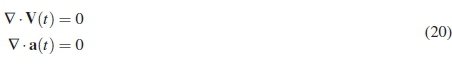
ABSTRACT
This paper derives the non-inertial terms, also referred to as fictitious forces, for aero-ballistic cases using an Eulerian approach. These cases display unsteady rates ofchange in acceleration in all six degrees offreedom. Six fictitious forces are identified in the momentum equation. Their origin and nature ofthese forces are elaborated upon. As shown in previous work, the continuity and energy equations remain invariant. The non-inertial boundary layer equations are derived to determine the effect of fictitious forces in the near-wall region. Through an order of magnitude analysis it was determined that none of the fictitious forces cancels out. It will therefore have an influence on the boundary layer properties.
Additional keywords: Coriolis force, Centrifugal force, Euler force, Magnus force, Reference frames, Galilean invariance, Rotational transform
Nomenclature
Roman
a Acceleration vector
b Vector
k Heat transfer coefficient
p Pressure
t Time
u Velocity vector
x Distance in x-direction
x Position vector
y Distance in y-direction
z Distance in z-direction
G Galilean operator
I Identity matrix
L Characteristic Length
O Frame designations
R Rotational transform operator
T Temperature
^ Rotational frame
V Velocity in x-direction
U Characteristic Velocity
X Position vector
Greek
δ Boundary layer height
ε Perturbation parameter
ε Internal energy
λ Second viscosity
μ Dynamic viscosity
ν Kinematic viscosity
ρ Density
ψ Pressure per unit mass
ω Rotational velocity component
Φ Dissipation Function
Ω Rotational speed around the z-axis
Ω Rotational speed vector
Sub- and Superscripts
' Orientation preserving frame
* Non-inertial frame
★ Normalised form
i Inertial frame
r Relative frame
rel Relative conditions
t Time
Δt Change in time
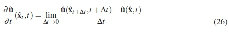
1 Introduction
Non-inertial implementation of the Navier-Stokes equations are mostly found in turbo-machinery applications [1,2]. This is limited to unsteady, pure rotation that operates at most in three degrees of freedom. Aero-ballistic and aeronautical applications make ue of six degrees of freedom and arbitrary motion. Inconsistencies have been found in the literature with regards to formulation of non-inertial flow equations for six degrees of freedom motion [3-5]. The Magnus force is absent from the momentum equations cited. Furthermore, there is uncertainty on the formulation of the conservation of energy equation. This paper extends on the methods used in [6-8] to obtain the non-inertial Navier-Stokes and boundary layer equations for arbitrary aero-ballistic motion.
The Lagrangian approach to deriving the inertial conservation of momentum equation makes use of Newton's second law [9]. This equation is rewritten to approximate the solution to momentum conversation of a fluid volume with the total derivative of the fluid parcel velocity on the left hand side of the equation.

In the non-inertial frame, acceleration terms are derived through a point mass method [9-11] to arrive at:
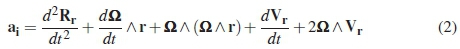
To obtain the correct non-inertial momentum equation, the time derivative of the non-inertial acceleration, (Vr) must be implemented in the total derivative equation as shown below [9].

The misconception have been observed that the acceleration terms in equation 2 can be directly applied in Newton's second law:

Coincidently this approach provides the correct set of non-inertial equations for rotational cases. It does not when six degrees of freedom motion is at play.
Equation 2 presents the majority of the fictitious forces associated with aero-ballistics motion; Coriolis force, Centrifugal force, Euler force and unsteady translation. In external ballistic models the Magnus force and a secondary force due to moving of the axis of rotation is included. At commencement of this work it was uncertain if these forces should be included in non-inertial fluid equations.
The physical meaning of the Coriolis force has been a subject of many discussions [12-14]. The Coriolis force was first mathematically formulated in 1835 by Gaspard Coriolis. Observations of the Coriolis effect on the surface of the earth long preceded the formulation (figure 1).

Deflections due to the Coriolis effect is three dimensional, but the term Coriolis force is mostly associated with horizontal deflections with respect to the surface of the earth in the Northern and Southern Hemispheres. This has specific application in Meteorology and Geophysics since weather patterns and sea currents are directly influenced by the horizontal component of the Coriolis force.
While the deflection on the surface of the earth has been the most general observation of the Coriolis force, the component vertical to the earth's surface has only been measured in 1908 by Lorand Eötvös [13]. He observed the effect through gravity readings collected by research ships which indicated that the gravity measurements increased with motion towards the west and decreased when the ships sailed in an easterly direction.
Although the Coriolis force is mostly explained in terms of, and therefore associated with, rotation of the earth it is applicable in any rotational system. It is especially important in ballistics research since earth rotation influence the accuracy of fire-and-forget weapon systems. The Centrifugal effect always accompanies the Coriolis effect. This is responsible for the outward motion of the flow in a rotational system.
The presence of the Magnus force in the non-inertial momentum equation is not generally seen in literature [9, 11]. Non-inertial formulations do not regularly include all the aero-ballistic accelerations and is generally applied to rotating flows. In CFD applications the Magnus force is mostly investigated using a predictive approach [15-17] instead of with prescribed motion on the non-inertial frame as suggested here.
The mathematical origins of the Coriolis, Centrifugal and Euler forces were determined in [6,7] for rotational cases. It is a result of transformation of the material derivative to the non-inertial frame. Insight is obtained in this paper to the origin of these non-inertial terms in aero-ballistic frames of motion. The physical meaning of the terms and if it will effect boundary layer profile is mathematically investigated here. This is done through derivation of the non-inertial Navier-Stokes and boundary layer equations by extending the methods used in [6,7].
2 Transformation between Absolute and Relative Frames
In this derivation the same three reference frames as used in [6, 7] will be made use of to transform the inertial Navier-Stokes equations to the relative form (figure 2). These frames comprise of:
• Frame O, which is an inertial frame. This frame is stationary.
• Frame O', which is a non-inertial frame. This frame is orientation preserving with respect to Frame O. It therefore has three degrees of freedom and is free to translate.
• Frame Ô, which is a non-inertial, rotating frame. This frame does not preserve orientation therefore it has six degrees of freedom. It can translate and rotate as predicted by the accelerations imposed on point P. This frame shares an origin with Frame O'.
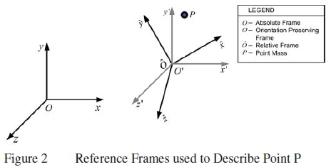
Consider the point P. The motion of this point can be described from each of the three frames. This point is in arbitrary motion.
The flow field that surrounds this point can be described from any of the reference frames. The standard Navier-Stokes equations hold in the inertial frame, therefore the objective is to obtain the correct form of the equations in Frame Ô. It will be accomplished by conducting two transformations.
The first transformation will account for arbitrary translation between the inertial frame and the orientation preserving frame. Since Frame O' and Frame Ô shares an origin, this transformation accounts for the translation of Frame Ô as well. A modified Galilean Transformation will be used to this effect.
The second transformation will account for arbitrary rotation. A transformation from Frame O' to Frame Ô will be defined. The relation derived during the first transformation will be used to describe the flow field in Frame Ô in terms of the vectors of Frame O.
2.1 Modified Galilean Transformation
The modified Galilean transformation as used in [6,7] is extended here to account for six degrees of freedom motion. Assume that the frame origins intersect at time t = 0 and that frame Ô is moving at velocity vrel with acceleration arel in three dimensional space. At time t = Δt frame O and O' are distance xrelfrom each other. The is depicted in figure 3.
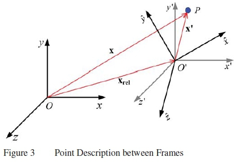
In figure 3 the absolute distance can be described in terms of the relative and non-inertial distances:

The relative distance between the two frames is a summation of the accelerating translation and rotation and is described by:
The relative velocity component consist of the translating and rotating velocity components so that:

In this equation the translation component is a function of time only as it describes the motion between the origins of Frames O and O'. The rotation is taking place in Frame O' and is therefore defined in this frame.
The acceleration is the time derivative of the velocity:

The first term represents the translational acceleration, while the second and third terms is a result of the rotational velocity. Since both the derivative of x and Ω is not equal to zero, these terms will contribute to the total relative acceleration. The accelerating component can therefore be expressed as:

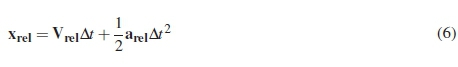
Equation 6 is a Taylor series expansion that was truncated after the second order term since constant acceleration was assumed. Had the acceleration not been constant, the additional terms would be accounted for by the inclusion of further derivative terms:
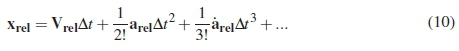
In this equation it can already be seen that the effect of higher order derivatives of xrel becomes smaller and smaller. In the subsequent paragraphs it will be shown that from the second order, the terms are negligible.
A description for the relative motion can be obtained by substituting equations 9 and 7 into equation 6. This will result in:

The relation between the order preserving frame and the inertial frame is defined through a modified Galilean transformation:

2.2 Rotational Transform
The rotational transform for this case can be defined as the projection of the vectors in the orientation preserving frame on the rotational frames. This is depicted in figure 4.

The vector components in Ô is related to O' by defining a rotational transform and substituting equation 19 to relate Ôto O:
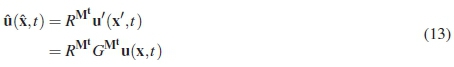
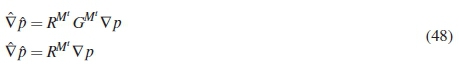
RMtis therefore the rotational transform that operates on X´ to obtain the  co-ordinates in the accelerating, rotational frame.
From equations 12 and 13 it can be derived that for the velocity vector the following relation holds:

3 Transformation of the Navier-Stokes Equations
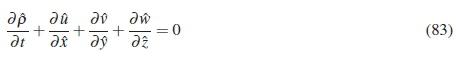
3.1 Continuity Equation
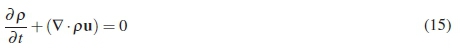
Consider the continuity equation in the inertial reference frame [9]:
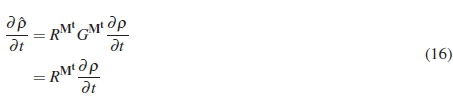
As scalars are invariant under transformation [18,19] the time dependant term in the inertial and accelerating frame is related by:
The relation of the second term in the continuity equation becomes:
With the implementation of equation 14 the relation is simplified to:
The divergence of a cross product is equal to zero, hence a number on the terms in the above relation is cancelled out:

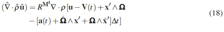
Furthermore, the divergence of the translational components are equal to zero. This is due to the translation being dependant on the time dimension alone - V(t) and a(t) are constant throughout the spatial domain at any given time step:
The relation is hence simplified to an invariant relation as all the additional terms cancels out:

The addition of equations 16 and 21 gives a relation for continuity in the non-inertial frame:

By implementing equation 15, the final equation for mass conservation in the accelerating frame is obtained:

It was shown in [6,7] that the continuity equation is invariant under transformation for rotational cases. Here it is mathematically shown that this prevails for arbitrary motion cases as well.
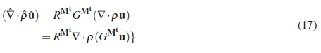
3.2 Conservation of Momentum Equation
The incompressible form of the momentum equation as shown in [6] and [8], made the assumption that the change in density is negligible. Therefore, the equation could be simplified by dividing density into all the terms as there are no temporal or spatial gradients in density. The diffusion term in particular could be simplified in a manner that would facilitate easy transformation where the divergence of the gradient of velocity yields the same result as taking the Laplacian of the velocity. This is not the case when compressibility has to be accounted for. The compressible Navier-Stokes equation in the inertial frame will take the form [9]:

The non-inertial form of the separate terms of the equation, will be derived from this form to obtain the compressible equations in the acceleration frame.
3.2.1 Unsteady Momentum Term Transformation
First consider the unsteady term in the non-inertial frame and apply the product rule for partial derivatives. This operation will result in two terms that was not considered during the incompressible case [6]:
The first transformation will concern the unsteady term where an expression must be found for:
The first task is to find an expression for the term  The expression will take a form that is similar to equation 13:
The Taylor series expansion for x,t+At is expressed as:

The expression above is as seen from the orientation preserving frame. Since this frame is free to translate, but not to rotate, only the rotation terms are relevant here. The equation above is truncate at the second order and with the substitution of the rotational components of equations 7 and 9 and further re-arrangement the equation becomes:

The Fourier series expansion is obtained for 
 . Substitute equation 29 into the expression to obtain:

The equation above is substituted into equation 27 to get the expression:
In order to complete the expression in equation 26 further definitions are required. The assumption was made that the point P is fixed in the rotating frame, and the rotation is around the object axis (meaning that O' and Ô share an origin), then the relation of motion between two time steps are:
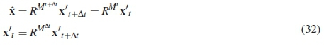
Next a Taylor series expansion for xt+Δt is developed and the equation above is used to arrive at:

Re-arrange the expression above and consider it in the limit yields:

If this expression is considered for any vector b, and taken into account that xt+At- xtas At - 0, the following equation related to rotation is obtained:
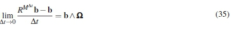
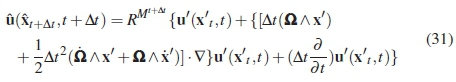
With all the required expressions in place equation 26 can now be completed:

Equation 35 is used to simplify the expression above and with some re-arrangement of terms the following expression is obtained:

This equation above will retain its current form irrespective of any further changes in acceleration. All other terms that is inserted to account for variation in acceleration will become negligible when the expression is considered in the limit.
Substitute equation 37 into equation 25 and with the aid of equation 13 and further manipulation the above becomes:

The product rule is then used to combine the terms  and
and  so that the equation simplifies to:
Equation 14 is substituted in the equation above to remove the modified Galilean operator from the equation:
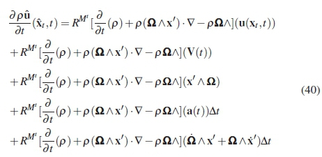
The different parts of 
 which is the third combination of terms in equation 40, will now be considered.
The transient term in the equation above can be expanded on with the use of the product rule for partial differential equations:
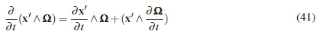
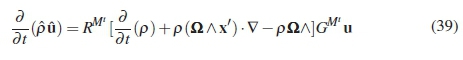
In the equation above the first term on the right hand side represents the unsteady motion of point P in the frame in cases where the rotation is not purely about the fixed axis. In pure rotation cases this term will be equal to zero. The second term represents the unsteady rotation, this is referred to as the Euler fictitious force.
The terms 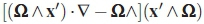 is equal to zero and cancels out:

The relation  will, for this case, simplify to:
The entire fourth combination of terms in equation 40 falls away, if not due to the mathematics, it will fall away in the limit due to the at term.
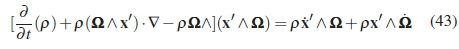
The above leads to the final description of the unsteady terms in the momentum equation for arbitrary acceleration:
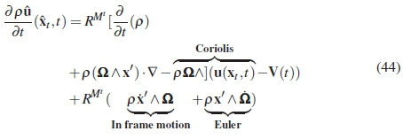
In any arbitrary acceleration case, this is the form the unsteady component of the equation will always take. Additional higher order terms that appear in the relative equations will become negligible in the limit due to the a.
Take note in this equation of the appearance of a part of the Coriolis effect and the Euler effect.
3.2.2 Advection Term Transformation
The relation between the frames for the advection term in the compressible Navier-Stokes momentum equation is:

By using equation 12 and the identity below the equation can be simplified.

This will lead to the following expression for relating the diffusion term in the non-inertial frame to the terms in the inertial frame:
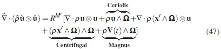
The original of the second part of the Coriolis and the Centrifugal terms can be seen here. Furthermore, an additional term that represents the change in diffusion due to the interaction between the translating and rotating part of the flow can be seen here.
3.2.3 Pressure Gradient Term Transformation
The pressure gradient term in the momentum equation is transformed. This part of the equation remain invariant since it is a scalar.
3.2.4 Diffusion Term Transformation
In the transformation of the diffusion term the difference between the compressible and incompressible cases must be noted. The divergence of the velocity vector is not negligible, therefore the completed diffusion term must be accounted for. The expression for relating the diffusion term between the frames hence becomes:

With the implementation of equation 14, the right hand side of the equations becomes:
If it is considered that,
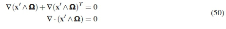
It can be shown that the diffusion component of the momentum equation is invariant for constant rotation conditions:

3.2.5 Final Transformation of the Non-Inertial Momentum Equation
The final transformation of the momentum equation relies on the summation of the transient and advection terms, as well as further manipulation of the resulting groups of terms.
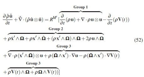
Group 1 is replace by the equation below, where equation 24 was used the rotational transform multiplied through the equation. Subsequently the non-inertial form of the terms were obtained:

The group 2 terms represents the majority of the fictitious forces. These were manipulated as shown below to determine the non-inertial form:

The remainder of the terms, group 3 conveniently cancels each other out.
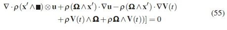
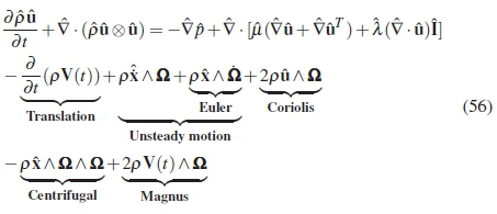
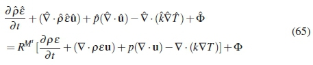
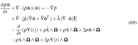
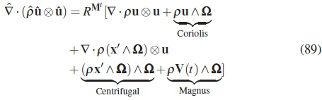
Summation of the transformed parts of the momentum equation lead to the final form of the compressible, non-inertial momentum equation for full arbitrary motion:
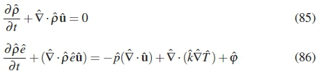
3.3 Energy Equation
Consider the energy equation in the inertial frame [9]:

The various terms can be transformed to the non-inertial frame separately and then combined to obtain the energy equation in the non-inertial frame.
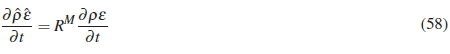
The time dependant term can be related between the frames as shown below since scalars are invariant under transformation:
The relation for the convective term between the inertial and non-inertial frame is shown below. This equation can be expanded upon with the used of equation 14:
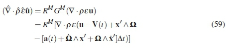
The second and third terms on the right hand side of the equation above was shown in equation 20 to be equal to zero. The convective term therefore becomes Galilean invariant under transformation:

The term that represents the rate of work done by the normal force can be related in the inertial and non-inertial frames as shown below. This term can be expanded upon using equation 14.
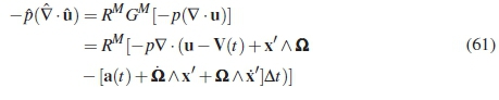
Showing that the second and third terms is again equal to zero, the same as above and indicated in equation 20, this transformation is also invariant.

The diffusive term in the non-inertial frame can be expressed in the inertial frame with the following relation:

Since k and T are scalars the relation is invariant under transformation:

The full relation between the non-inertial and inertial frames for the energy equation can be obtained by summation of the components obtained above. This leads to the equation:
The right hand side of the equation is equal to zero, this can be seen from re-arrangement of the terms in equation 57. The non-inertial energy equation is invariant under transformation in this specific case for constant acceleration in rotation [3], but it can be seen that this equation will remain in this form even if the acceleration is not constant. Equation 93 is further used to arrive at:
4 Boundary Layer Equations for Arbitrary Accelerating Flow
The Blasius solution to the flat plate flow is a classic solution to the boundary layer on a flat plate. Monaghan's solution [90] extended the solution to obtain an approximation for the flat plate boundary layer in compressible conditions. Extensive work was done by [1, 91, 99] to determine the boundary layer equations on rotating blades, but it appears that limited work has been done on boundary layer in arbitrary acceleration. In this section the boundary layer equations for the flat plate in arbitrary acceleration is derived (figure 5) in the same manner as indicated in [6].
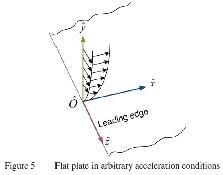
4.1 Flat Plate in Cartesian Components
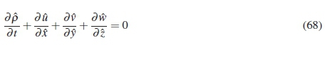
The continuity equation was derived in vector form in the previous section as shown in equation 93.

The component form of the equation is required for determining the boundary layer equation:
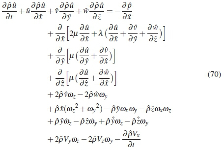
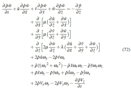
The momentum equation was derived in vector form in equation 56.
In component form the equation becomes as shown below for x-momentum, y-momentum and z-momentum respectively:

4.2 Non-dimensional and Perturbation Parameters
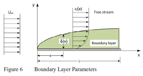
Partial differential equations are analysed by obtaining the non-dimensional form through scaling of the characteristic properties [9]. This allows for analysis of the relative magnitudes of the separate terms in the component form of the equation. The characteristic properties of a laminar boundary layer are shown in figure 6. It comprises of a reference length (L), reference velocity (free stream velocity U), boundary layer thickness (δ) and other free stream properties such as viscosity and pressure.
Scaling (see figure 7) is aimed at obtaining the relative sizes of the terms in order to identify smaller terms that can be neglected from the equation [23,24]. Elimination of the smaller terms result in a simplified equation. These equations contain the terms that have a significant effect in the near-wall region and are responsible for the behaviour of the flow in the boundary layer. The physical responses of the boundary layer to accelerating conditions are explained using the simplified equations.

The analysis is based on the assumption that the boundary layer thickness, δ, is much smaller in comparison with the body over which the flow is analysed [25],

A perturbation parameter, ε is introduced. This represents a very small disturbance in the flow at the surface that asymptotically approaches zero as indicated in figure 8.
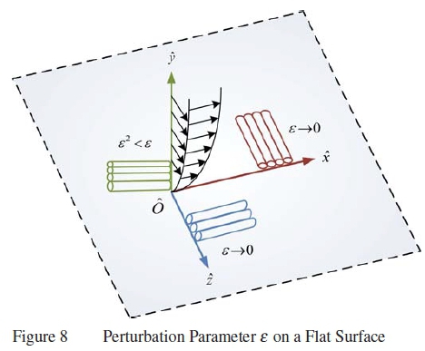
The perturbation originates from the surface of the plate continues to propagate along it. Therefore the disturbance approaches ε in both the x- and z- directions in figure 8. In the y-direction the disturbance approaches ε close to the wall, but it dissipates further way from the wall since the interaction of the fluid with the solid surface sustains the disturbance. At the flow boundary the disturbance is smaller than ε and of order ε2. The boundary layer height is smaller than the disturbance at the wall and asymptotically approaches ε2. It is defined that [25,26]:

In order to keep the solution as general as possible, it will only be assumed that velocity and time has positive values:
The non-dimensional parameters that is selected for the spatial variables is as follow:

L is the reference distance, the assumption is made that the plate is semi-infinite in the x- and z-directions. δ is the boundary layer height in the y-direction as a distance of L.
The velocity components are non-dimensionalised as follow, where U is the characteristic velocity:

The specific pressure and kinematic viscosity can be normalised as follow:

The angular velocity can be non-dimensionalised by multiplying it by t. The units of angular velocity is rad/s, but since radians are already a non-dimensional quantity it can be normalised in this manner.

4.3 Development of Boundary Layer Equations
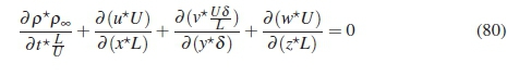
Applying the normalization parameters to equation 68 results in the non-dimensional form of the equation:
The equation above is multiplied by:

leading to the final non-dimensional form of the equation:
No terms can be neglected from this equation and boundary layer continuity equation thus remains the same as the equation for the bulk flow:
In a similar way, the boundary layer equations for the conservation of momentum equation can be determined.
Normalising equation 72 and simplifying as shown above, leads to the boundary layer equations for arbitrary acceleration on a flat plate:
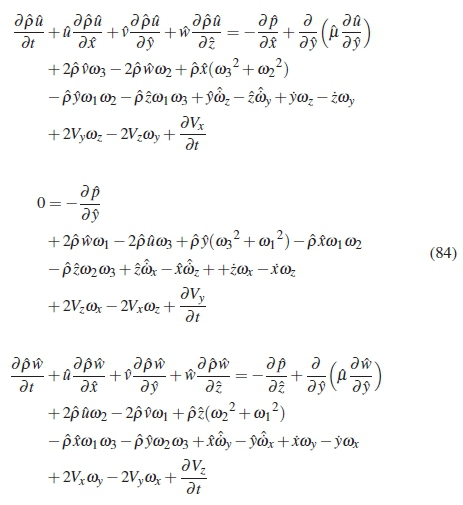
The above equations has in similar form as it would have had in the case of no acceleration, where the majority of the viscous terms becomes negligible. The difference is however in the presence of all the inertial terms since none of it becomes negligible. Acceleration of an object will affect the boundary layer due to the presence of the inertial forces.
5 Closure
There are a number of misconceptions that have been observed in literature with regards to flow equations in non-inertial reference frames. An example where discrepancies in the literature is seen is in the conservation of energy equation. Some sources add fictitious energy terms to these equations [4, 5]. It was shown through derivation that both the continuity and conservation of energy equations remains invariant under transformation - no additional terms are added to these equations:
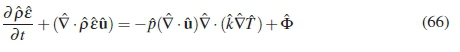
The equation for full arbitrary acceleration below indicates that there are six fictitious terms in the non-inertial momentum equation. These are the only terms that are present during arbitrary acceleration; the higher order terms become negligible or cancel out with other terms during the derivation. The equation for full arbitrary motion (six degrees of freedom) can be used to explore the appropriate form of the non-inertial momentum equation for steady translation and unsteady rotation.

The mathematical origin of the fictitious terms are observed during the derivations. The unsteady translation term, two terms due to unsteady rotational motion and the first parts of the Coriolis and Magnus terms originates in the transformation of the unsteady component of the momentum equation (equation 44).
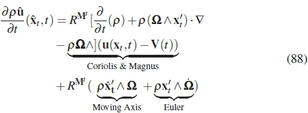
The remainder inertial terms, second part of the Coriolis, centrifugal and the term representing the interaction between the rotation and translation, all has their original in the transformation of the advection term (equation 47).
Observation of the effect of both Coriolis and Magnus effects can be explained using a mathematical approach which is seated in an understanding of the cross product operation. In figure 9 it is shown that a particle travelling in north on the earth's surface deflects to the right in the northern hemisphere and to the left in the southern hemisphere.

The difference in deflection is a function of the surface curvature of the earth where a velocity vector in the south has a different orientation than in the north. The result is that the cross product of the velocity and the rotation has a resultant force that is dependent on the hemisphere it operates in.
The Coriolis force is therefore described as a non-inertial force that operates on an object that is in motion relative to a reference frame. The effect of the Coriolis force is to cause deflection of the object in three dimensions in with a magnitude and direction that is determined by the cross product of the object's non-inertial velocity and the rotation of the frame, 2ρûλ Ω.
The Magnus force has a similar formula to the Coriolis force, but it has a different physical meaning. It is a function of the object's translation and represents the interaction between the rotating and translating motion of the object. It is therefore a non-inertial force that operates on a rotating object that is in motion relative to a inertial reference frame. The effect of the Magnus force is to cause deflection of the object (figure 10) in three dimensions with a magnitude and direction that is determined by the cross product of the object's transla-tional velocity and the rotation of the object, 2ρ V(t) λ Ω.
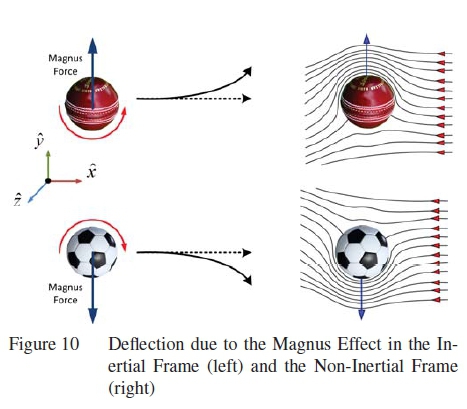
The presence of the Magnus force in the non-inertial momentum equation is not generally seen in literature [9, 11] since non-inertial formulations does not regularly include all the aero-ballistic accelerations and is generally applied to rotating flows. In CFD applications the Magnus force is mostly investigated using a predictive approach [15-17] instead of with prescribed motion as suggested here.
Acknowledgements
The authors would like to convey their gratitude to the following institutions for support in conducting this work:
1. Armaments Corporation SOC Ltd, South Africa.
2. National Research Foundation, South Africa.
3. Russian Foundation for Basic Research, Russian Federation.
References
[1] Bogdanova VV, Universal Equations of the Laminar Boundary Layer on a Rotating Blade, Flûid Dynamics, 1971, 6(9), 951-959. [ Links ]
[2] Dûmitrescû H, CardoA§ V and Dûmitrache A, Modelling of Inboard Stall Delay Due to Rotation, Joûrnal of Physics: Conference Series, 9007, 75(1), 019099. [ Links ]
[3] Diaz RA, Herrera WJ and Manjarrés DA, Work and Energy in Inertial and Noninertial Reference Frames, American Journal of Physics, 9009, 77(3), 970-973. [ Links ]
[4] Gardi A, Moving Reference Frame and Arbitrary La- grangian Eulerian Approaches for the Study of Moving Domains in Typhon, Masters Thesis, Politecnico di Milano, Spain, 9011. [ Links ]
[5] Limache AC, Aerodynamic Modeling using Computational Fluid Dynamics and Sensitivity Equations, PhD Thesis, Virginia Polytechnic Institute and State University, 9000. [ Links ]
[6] Combrinck ML, Dala LN and Lipatov II, Eulerian Derivation of the Non-inertial Navier-Stokes and Boundary Layer Equations for Incompressible Flow in Constant, Pure Rotation, Eûropean Joûrnal of Mechanics- B/Fluids, 9017, 65, 10-30. [ Links ]
[7] Combrinck ML, Dala LN and Lipatov II, Eulerian Derivation of Non-Inertial Navier-Stokes Equations for Compressible Flow in Constant, Pure Rotation, 11th International Conference on Heat Transfer, Fluid Mechanics and Thermodynamics - HEFAT 2015, Kruger National Park, South Africa, 91-94 July, 9015.
[8] Kageyama A and Hyodo M, Eulerian Derivation of the Coriolis Force, Geochemistry, Geophysics and Geosystems, 9006, 7(9), 1-5. [ Links ]
[9] White FM, Viscous Fluid Flow, Third Edition, McGraw- Hill, 9006.
[10] Batchelor GK, An Introduction to Fluid Mechanics, Cambridge University Press, Cambridge, 1967.
[11] Meriam JL and Kraige LG, Engineering Mechanics Dynamics, Fifth Edition, Wiley, 9003.
[19] Dolovich A, Llewellyn EJ, Sofko G and Wang YP, The Coriolis Effect - What's Going On?, Proceedings of the Canadian Engineering Edûcation Association Conference, June 90, 9019.
[13] Persson AO, The Coriolis Effect: Four Centuries of Conflict between Common Sense and Mathematics, Part I: A History to 1885, History of Meteorology, 9005, 9, 1-94. [ Links ]
[14] Thornton ST and Marion JB, Classical Dynamics of Particles and Systems, Fifth Edition, Brooks and Cole Publishers, 9004.
[15] Silton SI, Navier-Stokes Predictions of Aerodynamic Coefficients and Dynamic Derivatives of a 0.5 cal Projectile, Proceedings of the 99th AIAA Applied Aerodynamics Conference, 9011.
[16] Weinacht P, Stûrek WB and Schiff LB, Navier-Stokes Pre dictions of Pitch-Damping for Axisymmetric Shell using Steady Coning Motion, Army Research Laboratory Report ARL-TR-575, (1994)
[17] Cayzac R, Carette E, Denis P and Gûillen P, Magnus Effect: Physical Origins and Numerical Prediction, Journal of Applied Mechanics, 9011, 78(5), 051005. [ Links ]
[18] Kleppner D and Kolenkow RJ, An Introduction to Mechanics, Cambridge University Press, Cambridge, 9010.
[19] McCaûley JL, Classic Mechanics, Transformations, Flows, Integrable and Chaotic Dynamics, Cambridge University Press, Cambridge, 1997.
[20] Monaghan RJ, An Approximate Solution of the Compressible Laminar Boundary Layer on a Flat Plate, A.R.C. Technical Report 9760, UK, 1949.
[21] Dwyer HA, Calculation of Unsteady and Three Dimen sional Boundary Layer Flows, AIAA Joûrnal, 1973, 11(6), 773-774. [ Links ]
[22] Mager A, Laminar Boundary Layer Problems Associated with Flow Through Turbomachines, PhD Thesis, California Institute of Technology, 1953. [ Links ]
[23] Patankar SV, Numerical Heat Transfer and Fluid Flow, Hemisphere Publishing Corporation, 1980.
[24] Versteeg HK and Malalasekera W, An Introduction to Computational Fluid Mechanics: The Finite Volume Methods, Longman Scientific and Technical, 1995.
[25] Schlichting H, Boundary-Layer Theory, Third Edition, McGraw-Hill, 1968.
[26] Rogers DF, Laminar Flow Analysis, Cambridge University Press, Cambridge, 1999.
Received 9 September 2015
Revised form 27 December 2016
Accepted 20 October 2017

