


Serviços Personalizados
Artigo
 Inglês (pdf)
 Artigo em XML
 Referências do artigo
Indicadores

Links relacionados
-
 Citado por Google
 -
 Similares em Google
Compartilhar

 Permalink
Journal of the Southern African Institute of Mining and Metallurgy
versão On-line ISSN 2411-9717
versão impressa ISSN 2225-6253
J. S. Afr. Inst. Min. Metall. vol.124 no.3 Johannesburg Mar. 2024
http://dx.doi.org/10.17159/2411-9717/2681/2024
COMPUTATIONAL MODELLING PAPERS
Pragmatism in industrial modelling: An application to ladle lifetime in the steel industry
S.T. Johansen; B.T. Levfall; T. Rodriguez Duran; J. Zoric
SINTEF, Norway
SYNOPSIS
A methodology for building pragmatic physics-based models is here adapted to predict the erosion of ladle linings in the steel industry, in order to support operators when deciding whether the lining can be used safely for another heat. A defective lining may allow 140 t of molten steel to spill, with disastrous consequences for workers and plant. The adopted work flow for the development, challenges faced, and some model results are presented. One key learning outcome is that model development should allow time for maturing the process understanding, as well as for many iterations by 'questions-responses and actions' at various stages in the model development. Good interaction between the development team and industry case owner is an important success factor. Combining or extending the model with the use of machine learning and cognition-related methods, such as knowledge graphs and self-adaptive algorithms, is discussed.
Keywords: pragmatism, physics-based model, ladle lining, steelmaking.
Introduction
Many industrial processes involve complex physical and chemical systems. In addition, the observability (Wikipedia, 2022a) may be very poor and accordingly process control becomes difficult. In high-temperature processes, including the metallurgical industry, we find many representative cases. One example is aluminium reduction cells (the Hall-Héroult process), where the alumina concentration in the cell is measured by manual sampling once a day at a fixed location. This is the most important control parameter for a cell. Another example is from the ferro-alloy industry, where electric furnaces may have an installed power of around 40 MW. Due to the high temperatures of the charge (up to 2000°C: Jayakumari and Henning, 2020) there are no sensors capable of monitoring the interior state of the furnace. Sensors may be available in specific cases, but these are generally extremely expensive to purchase and maintain. Physics-based models can provide an alternative method for predicting the internal states of the process, if based on a realistic set of assumptions and simplifications. The amount of data in these types of processes is limited, and some of the data may have significant issues as a result of operational challenges. The operations are not automated, and sometimes fast decisions must be made without time to check if the change in operation impacts the data collection. In response to these challenges we have been developing a generic methodology (Johansen et al., 2017; Johansen and Ringdalen, 2018; Zoric et al., 2015a, 2015b), termed 'pragmatism in industrial modelling', for the development of industry-applicable physics-based models.
Earlier work on pragmatism (Johansen et al., 2017; Zoric et al., 2015a, 2015b) addressed solutions to various industrial tasks and problems. Here the best approaches were proposed and discussed, by assuming no limitations in human expertise and resources. A generic scheme for our pragmatic development approach is shown in Figure 1.
The use of the pragmatic modelling paradigm is aimed at handling the complexity of a hybrid modelling approach (a combination of data-based and physics-based modelling techniques in the same work flow) by:
1. Structuring the exchange of data and information between sub-models (often at different levels of abstraction)
2. Structuring the modelling and analytic work flows
3. Providing good interfaces to include some machine learning (ML) or artificial intelligence (AI) prediction tools (also in cases where the analytical or computational physics models are more tightly integrated with AI/ML tools)
4. Connecting these various tools to the relevant decision support tools and processes.
The inclusion of modelling and simulation frameworks in industrial processes and decision support systems requires significant structure and standardization, which we hope to contribute to by this work.
Pragmatic modelling starts always with a given industrial application, by defining an industrial use case (i.e. problem to solve) (Wikipedia, 2022b). The pragmatic model is the simplest model that can give fast and sufficiently accurate answers. There could be a short step from a pragmatic model to online process control and operation support tools. A pragmatic model starts with the simplest possible model that has a value for the user. The main steps of the pragmatic work flow are shown in Figure 1:
1. Problem and context identification
2. Analytical strategy and plan
3. Architecture of the analytical framework
4. Execution (coordination of analyses, simulations, and experiments)
5. Evaluation of the solution
6. Conclusion and communication.
A key element in this work is the appointment of the system architects team (Zoric et al., 2015a, 2015b; Wikipedia, 2022c; 2022d), as the capabilities of this team will be a critical factor for a successful outcome of the work.
The methodology, which the system architects team has to orchestrate, is not limited to any specific techniques (steps 2-4), and the palette of tools may contain elements that involve mathematical methods, such as statistical methods, singular value decomposition (Wikipedia, 2022e), and reduced order methods (Wikipedia, 2022f) as well as numerical continuum physics, numerical particle physics, and molecular and quantum mechanics. In practice the system architects team will learn to apply and orchestrate the methods that are at hand for the development team (methods applicable to the reality of the industrial process, and related decision support systems and routines), and AI should already be included in the abovementioned methods. The pragmatism-based methodology will use available sensor data and assess the validity of the data. However, development of new sensors, even if critical, is not dealt with by the methodology.
In this paper we aim to present a simplified pragmatism-based approach for the development of a prediction model for steel ladle refractory erosion and lifespan. A particular challenge is that the total development team is small (2-3 people) and multiple trade-offs must be made to develop a useful model in a limited time.
Context of the COGNITWIN project
This work, as a part of the Horizon 2020 project (COGNITWIN, 2022), is aiming at accelerating the digital transformation and introducing Industry 4.0 to the European process industries. The project is focused on six industrial pilots, ranging from aluminium, silicon, and steel production to engineering. Here we address the pilot for the Sidenor1 steel company, where we analyse how to increase the ladle refractory lifespan, and how the digital twin concept can contribute.
Sidenor ladle case description
Steel production in the melting shop process is based on three main steps. The first involves the production of liquid steel by smelting iron ore in a blast furnace (BF) or melting scrap in an electric arc furnace (EAF) or induction furnace. The second step - secondary metallurgy (SM) - is necessary for refining the liquid steel, and the last one solidifies the steel during ingot or continuous casting processes.
Typically, a ladle can contain from tens to hundreds of tons of liquid steel (Figure 2). Most ladles have a porous plug at the bottom. Gas (Ar of N) is injected through the plug to stir the liquid steel.
The bubble driven upward flow of the liquid steel promotes the transfer of inclusions from the steel to the slag and homogenizes the temperature and chemical composition.
The main objective of SM is to obtain the correct chemical composition and to ensure an appropriate temperature for the casting process. In addition, there are several important tasks which must be complete during SM, for example removal of inclusion and gases. In order to reach these objectives, Sidenor has a SM mill consisting of two ladle furnaces (LFs) and a vacuum degasser (VD). Each LF has three electrodes for heating the slag, steel, and ferro-additions. The ladle contains liquid steel and slag for all the production process, from the EAF to the end of the casting process. The liquid steel has a temperature of around 1850 K in the ladle and it is covered with slag, which prevents contact between the liquid steel and the atmosphere. The slag has a lower density than steel and consists mainly of lime and various oxides. Slag conditioning can be improved during SM by adding slag-formers.
In order to handle the liquid steel and slag at such high temperature, the ladle is constructed with a strong outer steel shell, the inside of which is lined with layers of insulating (refractory) materials. The refractory consists of ceramics and its most important properties are:
i. Ability to withstand high temperatures
ii. Favourable thermal properties
iii. High resistance to erosion by molten steel and slag,
The inner layer of refractory bricks, which are in contact with the liquid steel, and slag, is progressively eroded by each heat, and after several heats the erosion is such that it is not safe to use the ladle for another heat. The refractory is visually inspected after each heat and depending on its state, the ladle may be used again, or put aside for repair or demolition. In case of repair, the upper bricks, which are more eroded, will be replaced and the ladle is returned to production. Later, based on continuing visual inspection, the ladle may be deemed ready for demolition. In this case the entire inner lining is replaced.
One important goal for Sidenor is to reduce the refractory costs by identifying new methods for extending the refractory life. One of the key aims is to use the same ladle for more heats without compromising safety, but another important issue is to better better understand the mechanism that underlies refractory erosion and avoid as much as possible the working practices that shorten the usable life of the lining.
Target for the pragmatic model development
The main goal of our pragmatic modelling approach is to develop a model from which the results can help decide whether the ladle can be safely used again without repair or relining. The model should incorporate both historical and current production data. The model should increases the knowledge of the operators, and could also contribute to related digital twins in semantic and cognitive aspects.
In addition, the model should provide information about which parameters contribute the most to ladle refractory erosion, and what precautions can be taken to extend refractory life.
Physics-based pragmatic model
We now investigate the recommended work flow for the development of the abovementioned pragmatic model. The generic work flow could be applied to the development of any physics-based models. A particular ambition with this work is to develop a hybrid model that can base predictions on any combinations of direct use of data, indirect use of data, and the physics-based model. However, for the physics-based model the data is crucial for tuning the model. The justification of tuning is that we are dealing with an extremely complex process, containing multiple levels of uncertainty. As part of the overall complexity many aspects of critical physical data are unknown or have changed due to ageing.
It was decided to frame the model as PPBM (pragmatism in physics-based modelling). Referring to the pragmatism steps 1-6 above, we first set out to establish the development team, comprising mainly two developers. This step is preparatory, and the team was selected based on experience and skills. In addition, the contributions from the industry were crucial for understanding the case and providing relevant data.
The following text describes the PPBM development in six steps, as illustrated in Figure 1.
Pragmatism step 1: Problem and context identification
Step 1 aims at describing accurately the purpose of the model and the quantitative output data the model shall produce, including time constraints and accuracy requirements. To facilitate this step we employ the user experiences described from the perspective of ladle operators at Sidenor. The main user, who is expected to benefit from the model results, places the model in the industrial perspective and defines its role and contribution to the industry process. We discuss our experiences in solving the challenges met during that collaboration, which we experienced as very demanding. The actors and entities participating in the overall case work flow are shown in Figure 3. The step (1) Definition Accepted should have been finished at latest after 6 months. However, the problem definition and context were continuously challenged without any formal requests to change the definition. In addition to developing the physics-based model the objective included developing the model in such a way that it can be used in different hybrid approaches, combining data and physics-based models. The hybrid approach, involving using data to calibrate the model, is included here, while development of models that explore the combination of the physics-based model and all additional available data is outside the scope of this development. However, continuous interaction between the ML team (MLT) and the physics-based team had to be ensured. Important decision gates during the model development process are illustrated in Table I.
User story
The main output of this phase, the user story, can be summarized as a model of the SM that can predict the average refractory loss for a given use of the ladle, and the accumulated loss over the lifespan of the ladle. The expected input paramesters are the amounts of steel, slag, and additives held in the ladle. Predictions of the temperature of the steel, slag, and refractory wall are important determinants of refractory loss. We therefore need the temperature in the steel as hot steel is added to the ladle. To account for heating during SM we need the electrical power that is input as a function of time. In addition, we need the time history of applied inert gas and the vacuum pressure above the melt. The model must be able to take the entire history of the ladle (since the last relining) into account when the simulations are run. The state of the refractory wall from the previous heat, in terms of temperatures and erosion, must be input to the next use of the ladle (next heat). It should be possible to continue the simulation when new data is available.
Pragmatism step 2: Analytical strategy and plan
This part of the development included overall model design, resulting in a specification document. This document was very detailed, but still only a signpost towards the implementation. Instead of writing a specific implementation report the code included necessary comments and the original specification was updated when changes were made. As regards the functionalities (how to use the model) no specific documentation was completed apart from short text files to explain the scripts.
The ladle and refractory, with bottom porous plug and tap-hole, is three-dimensional. To develop a fast model that can simulate the refractory behaviour over weeks in real time, using a full 3D model, and with the available time and resources, was deemed infeasible.
However, many of the ladle's features can be represented in a simplified 2D model. It was therefor decided to move on with a 2D model.
The model simplifications are listed below.
> During part of the ladle operation the ladle is inside a ladle furnace (SM mill) with electrodes (for Ohmic heating) immersed in the slag. The electrodes have a heating efficiency (tuning coefficient) and dynamic effects of heat storage in the electrodes are neglected. However, it was subsequently learned that the electrodes do not contact the slag or metal, but supply heat via arcs between electrode tip and slag/metal. The arcs radiate towards the refractory bricks placed above the level of liquid steel and slag. This radiation may be excessive in some cases.
> The additions to the ladle will need time to melt and mix. It is assumed that the melting and mixing processes are instantaneous. As a result, the model will predict an immediate temperature drop when additions are made to the melt, while in reality this cooling effect will manifest over several minutes.
> Vertical heat conduction between the bricks and inside the steel casing is neglected.
> Steel and slag temperatures are represented by mass averages.
> When hot steel is teemed into a colder ladle thermal cracking will occur, increasing with increasing temperature difference. These effects are very hard to model in detail and are proposed to be dealt with as a hybrid extension of the model.
> Excessive erosion of refractory above the slag/metal level is due to the extremely high temperature of the electrode arcs, together with irregular splashing of hot metal during vacuum treatment. These erosion phenomena, taking place above the average melt surface, are not included in the model.
Effects which are dealt with are dynamic temperatures in the side and bottom refractory bricks, insulation layer, and steel shell. When stirring gas is injected 2D CFD simulations were performed to compute the distribution of wall shear stresses. In Figure 4 we see an example from a 2D simulation of the gas-driven flow in the ladle containing both steel and slag. The maximum velocity is around 0.9 m/s, using a typical gas flow rate that has been used by Sidenor. The broken lines show trajectories of gas bubbles released from the bottom plug. The methods used here are Lagrangian representation of the bubbles, which expand due to the lower hydrostatic pressure and vacuum above the melt interface. The slag motion is represented by the volume of fluid technique (Wikipedia, 2023).
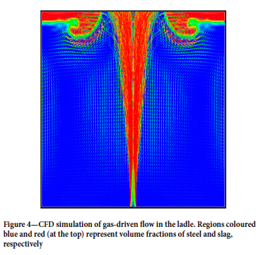
Based on a set of these CFD simulations the wall shear stress as function of gas flow rate and relative height could be extracted and used as input for heat- and mass-transfer models. Based on visual observations from video taken at the plant at a late stage of the project, it was found that application of the vacuum, together with gas stirring, led to a violent agitation in the steel close to the surface. This observation resulted in recalculations with CFD to account for gas expansion due to the local steel pressure. The result was much higher shear stresses close to the surface when vacuum was applied. New fitting functions for the wall shear stress as result of relative height, gas flow rate, and pressure above the steel were created and implemented in the model. It is noticed that when other team members visited the plant earlier in the project, the consequences of vacuum treatment on gas stirring was not realized and brought forward to the system architects team.
It was assumed that the slag behaved like a moving 'lid', floating on top of the liquid steel. The modelled wave agitation of the slag, caused by the gas stirring, provided an added local mass transfer rate for refractory dissolution into the slag. The assumption of the slag behaving as a lid should later be relaxed. This will, however, require more complex and time-consuming CFD work. This would improve the model in the slag-metal transition region.
Sub-models for refractory dissolution and erosion of the steel-wetted refractory, as well as dissolution into the slag, where it is present, had to be developed. Data for solubility of refractory binder in the steel, and for refractory solubility into the slag, was obtained from the literature and from thermodynamic equilibrium software (FactSage). The energy equations for slag and steel were written in terms of enthalpy, allowing for any relationship between temperature, composition, and enthalpy. This is important when dealing with cold additions to hot slag and steel.
Pragmatism step 3: Architecture of the analytical framework
Step 3, the architecture of the analytical framework, incorporated the designs of both the experiments, data structures and related analyses, and model and simulation entities in greater detail. After this step the development team should be ready for coordination of the experiments, analyses, models, and simulations and data/ information exchange among them. Of course, this phase is usually carried in several iterations, usually starting with the proof-of-concept model (simplest possible representative model), which gradually approaches the final result, i.e. the framework ready for execution of the work flows (step 4).
The architecture of the model was created in phases. In the first phase, a simplified proof-of-concept model was quickly implemented (as a monolithic approach) to see how the specification was holding up, and if more input was required. This proved valuable, as several issues were handled early. Python was chosen for building the model.
Once the basic model was working satisfactorily, the implementation was redesigned as a set of modules with well-defined interfaces to give the required flexibility in future applications of the model. We needed a model that could keep its state and be flexible enough to enable changes without major rewrites. The model itself was implemented as a single class, which proved valuable as we had to do several rewrites to accommodate unforeseen changes. The use of the model was set up as a series of input scripts, executing runs for the LadleModel object, and with different purposes. For instance, (i) running a single case, (ii) tuning the model with a set of parameters based on one or many cases, and (iii) running entire campaigns from first use till demolition.
The data was originally given as column-based data files (MS Excel and csv). In order to efficiently utilize the data, we had to pre-process it to fit our needs. For instance, the time-dependent data was given as large chunks containing multiple heats. These were split into one file for each heat. Later, the data was uploaded to a database (InfluxDB)2, and the data reading had to be changed to accompany two different sources. With hindsight it would have made sense to use a database in the first place. The output of the model was handled as a mix of plots, output to screen and the results saved to file. For the data from a database, the results were written back to the database.
Data was originally provided as csv files. At a later stage, data was loaded into InfluxDB. Doing this at a much earlier stage could have saved time. The database was chosen by external parties and was not a design choice for the pragmatic model (the modelling framework is quite generic and several other, standard database solutions could also be used).
Description of model implementation
The physics-based model developed here is implemented in Python as a single class. This enables a complete state of the model to be saved to disk and continued at a later stage. This is important as the final version will model several different steel ladles in parallel. Each heat-run of the ladle that should be simulated depends on the previous modelled state. As the simulation time is specified to be significantly shorter than one hour (seconds in reality), while each lade is used two or three times a day, we need to be able to start and stop the simulation easily.
The main ladle model depends on several stateless sub-models, all described in Johansen, L0vfall, and Rodriguez Duran (2023).
The model is reliant on both static and transient data from the plant. The data can be retrieved either from an InfluxDB database or from files on disk. Either way, data retrieval is relatively time-consuming, and is therefore done only when necessary, and the required data is stored inside the object and used when needed. When a new heat-run is simulated, a new set of data must be loaded, and the previous data-set is overwritten. Since the data will be loaded several times for the same object, it is loaded independently from the model initialization.
Depending on the model scenario, the same model with the same data could be run several times. For instance, the time from when casting is finished to when the ladle is filled with steel again is modelled as an empty ladle. This is done before the model is run again, but this time the full model and data is used. This way of using the model requires the possibility of resetting parts of the ladle state between the different runs. The temperature in the ladle wall, for instance, should not be reset, but parmeters like the amount of steel and simulation time should be reset.
The actual simulation of a specific heat for a of the steel ladle is carried out with constant time-steps. First, a preparatory step is done, where the amount of steel and slag in the ladle is determined, the heat added to the ladle during the time-step is calculated, and the gas flow rate and pressure are extracted from the data. In addition, the fraction of steel and slag for each cell is determined, and the mass lost from the refractory during the time-step is calculated.
Next, the new temperature in the steel and the slag is solved for. With this given, the temperature in the wall and the bottom layer is calculated. Once the model is solved, time-dependent data is stored inside the object before the next time-step is carried out.
The mass loss (erosion) of the wall is calculated, and accumulated for each time-step, but the wall is eroded only at the end of each heat. Due to the different modes that the model is run in, the actual wall erosion is controlled from the outside as an explicit call to erode the wall. This is done to ensure that the temporary runs to create the correct wall temperatures do not affect the wall thickness.
The model should always be used with an external script that sets up a given scenario to be run. How the scenario is set up has a large impact on the results.
After a ladle is re-lined, it is used many times (40-50) before parts of the refractory are replaced. The ladle is then used until the entire lining needs to be replaced. Between each use of the ladle, the wall is not allowed to cool down (if the waiting time is too long the refractory is heated with burners, although this is not included in the model), thus the state of the refractory wall at the end of one heat and the waiting time until it is used again are both important for the next simulation. All must be taken into account when a simulation is run. This is done by allowing the user to control the model from the outside.
When a ladle object is created, no data is read into the object, therefore running the model at this stage would fail. This avoids having several ways to set the data, and enables the same object to be used for consecutive heats without copying results.
To show how this can be done, we will go through a couple of different scenarios.
First of all, it is important to be able to run a single heat independently, and to reproduce the results quickly. This way of running will not take the history of the ladle into account properly, and we need a way to estimate a realistic initial state for the refractory wall.
First we have a method to set the initial wall temperature (so as not to start from a totally unrealistic state, which would require a long simulation time to obtain a realistic result). This method will yield a linear temperature profile between the inner and outermost bricks. After reading the relevant production data into the case, we can run the case for a given amount of time to heat up the refractory to a realistic temperature. From the time that casting is finished to the next heat, the ladle will stand idle and the refractory will cool significantly. To account for this, we can run the model without steel and slag for a given time. The model will not be able to solve all the equations properly, and so a flag is set, telling the model that the simulation is run with an empty ladle. The ladle state is now ready to run the actual simulation. Due to the different modes described above we have an additional method to actually erode the ladle wall at the end of the simulation. This is to make sure that the temporary simulations are not changing the refractory thickness.
A more realistic scenario is to simulate an entire lifespan of a ladle. This can be done in much of the same way as described above. For the first heat, the recipe will be identical, while for the subsequent heats we can use the results of the previous heats as the initial state of the refractory. In this case we can also take into account the actual time between successive heats, as the waiting time between heats is recorded. This is now used to calculate how long the ladle is empty. Sometimes the waiting time is so long that a burner has to be used to keep the refractory wall warm. This is not simulated, and therefore we ignore waiting times longer than three hours.
We had an additional challenge; the initial temperature of the steel in the ladle was unknown. The temperature of the the EAF was available, but we found that this is not always representative of the starting state. To compensate for the unknown steel temperature, we iterate to find the initial temperature that results in the smallest difference between the calculated steel temperature and the measured temperature.
Pragmatism step 4: Execution
Step 4 coordinates work flows of experiments, models, and simulations and executes related data analyses. Ideally it should be possible, without any framework changes, to repeat the exercises and include them as an integral part of the industrial process. However, usually analyses in the evaluation step (step 5 in Figure 1) require repeating steps 3-4 until the framework reaches the quality needed for support of the industrial process.
The model exemplifies hybrid modelling, where we exploit both static data and dynamic data. Static data includes ladle materials, geometry, last temperature before it is filled with metal, time for repair of the refractory, and total number of heats before full relining of the ladle. At both relining and demolition (full relining) the erosion profile in the ladle was mapped. Dynamic data includes gas purging, vacuum evolution, heater power, steel temperatures (probe-based), alloy and slag-forming additions, time of tapping, and idle time until next heat.
The output data from the process is the measured steel temperatures and the data for relining and demolition. The number of heats before relining and demolition depends on the operator's visual assessments. The erosion profiles are maximum values and must be compared with the predictions, which are ensemble averages.
The execution step was found to be far from linear as it must involve multiple iterations. Based on initial execution of the model, using available input data, several issues regarding poor representation of data were found. As we see from Figure 3, decision point 5, when the model fails to reproduce data, we backtrack and update the model specification. This process was repeated many times throughout the project.
A good example of industrial data not always reflecting what might be expected is the steel temperature data reported by Sidenor. The logging system reports a new temperature every second, but from the data we could see that the temperature was constant for a long time, and then suddenly jumped. We quickly confirmed with the industrial partner that the logging system would repeat the last temperature value entered until there was a new value. In practice the temperature was measured at irregular intervals during the heats. We compensated for this by making a linear interpolation between the measured points. The temperature series is used to compare the calculated values with the measured, but is not used as input to the model, with one exception. The first temperature point was used as a starting value for the steel temperature in the ladle.
As the model improved, and we started running more cases, we realized that the first temperature sometimes seems inaccurate. For instance, we found cases where the temperature increased without any energy being added. Further investigation revealed that the first temperature 'measured' for a heat was the last temperature from the previous heat. We thus had no value for the critical starting temperature in the ladle. Temperature measurements from the EAF proved unsuitable for use as a starting value. We then decided that the best way forward was to iterate on the steel temperature by using the EAF temperature as a starting value, and minimize R0 (see Equation [2]) to a given tolerance, chosen to be 10 K.
To improve the model, we defined a set of tuning parameters. We then simulated the erosion state and temperature of the ladle continuously over many heats, until the maximum erosion of the refractory was 75%. This can be compared with the dynamic measured steel temperature in each heat, as well as the number of heats that was run until repair was necessary.
Another critical input for the numerical model is the amount of steel in the ladle. This is given in the data, but we found that sometimes the results from the numerical model gave a poor match with the data, and the reported amount of steel seemed either too high (more steel than the ladle can hold) or very low. By going through the steps of pragmatic modelling, we found out that the reported amount of steel in the ladle was what was cast, and not a direct measurement. Casting issues occasionally result in a cast being aborted. This will result in the reported steel weight being less than that actually used in the refining. The remaining steel will then end up being registered to one (or several) later heats. There is no way for the numerical model to compensate directly for these errors, as was done for the steel temperature. To avoid over-large discrepancies, we limit the minimum and maximum amounts of steel added to the ladle.
Tuning parameters that were selected were (i) refractory conductivity, (ii) melting heat for each addition, (iii) heat transfer coefficients (external, external emissivity, metal-wall, slag-wall, metal-slag, and slag, refractory and lid emissivity), (iv) electrode energy efficiency, and (v) carbon diffusion length in wear bricks. Here only the latter deals purely with erosion.
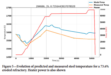
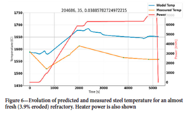
During testing of the model, it was found that the erosion state of the refractory and the evolution of temperature were closely coupled. In Figures 5 and 6 we see that the steel temperature is higher for a relatively uneroded refractory than for an eroded one. This is a result of a lower heat capacity in the eroded refractory. As expected, it was found that when the refractory was cold at the time of filling, the steel temperature is lower and more heating power is needed.
Temperature tuning was done in two steps, using a preliminary and approximate erosion model. As we found that the initial measured temperature in the data was not relevant, we also needed a strategy for obtaining a relevant initial temperature for the steel. Fortunately, we had measured temperatures from the EAF that could be used, when available. A temperature drop due to transfer of the steel had to be assumed.
Tuning step (a)
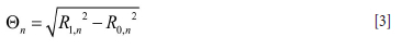
RMS residual for temperature was defined as
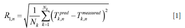
Here n expresses a campaign number and Nk (k = 1, .., Nk) is the number of temperature measurements in one heat. Now, if the initial steel temperature is incorrect that will drive a large residual R1,n. However, this problem is picked up by the residual R0,n defined as
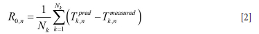
If the predictions are perfect we have, due to incorrect initial temperature for the steel, that
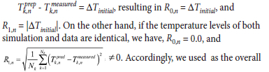
residual to minimize:
Tuning step (b)
Here we correct the initial temperatures in order to obtain the correct steel temperatures for the simulation of refractory erosion. Based on step (a) the initial temperatures are corrected for all cases where |R0,n| > 10 K.
Note that in both steps (a) and (b) the erosion is predicted based on preliminary tuning. As the refractory is eroded this will also impact the thermal dynamics of the system.
Tuning step (c)
Now we tune the erosion part of the model. We have data on when a decision was taken to repair the refractory and when it was demolished.
We do not have a model for degradation due to thermal shock, and this element is for now not considered. As thermal shock is most important at the bottom of the ladle, while chemical erosion is most pronounced at the slag line, this omission may not be critical for the usability of the model. Accordingly, we tune the erosion part of the model to match the observed number of uses until repair.
Repair is deemed necessary when the maximum erosion is greater than 75% for the three inner bricks.
We have here a new residual, Θrepair,n to minimize.

Here N represents the number of heats and n is the campaign number.
Tuning step (d)
When we can reproduce the times of repair well, we move on to reproduce the number of heats before demolition. In a ladle repair the bricks above a given level are repaired, while those below are not repaired. This must also be considered for the tuning. Optimally, we should find that tuning of the demolition is not required. However, it is possible for a repair to change the properties of the refractory in a way that necessitates some tuning of the models to handle the evolution of erosion after repair.
In this case it was eventually found that no tuning behind step (c) was necessary. The model could reproduce the demolition data very satisfactorily.
Pragmatism step 5: Evaluation of the solution
The outcome of the development is twofold. We have a model that can deliver certain prediction results. In addition, we have a numerical code that can be utilized as an element in multiple applications such as cognitive digital twins and other applications for asset management and optimization.
The quality of the solution is in this case exemplified by a comparison between prediction and measurements at the time of demolition, for all ladles and ladle campaigns operated by Sidenor in 2019. The result is shown in Figure 7. The averages are carried out over bricks 7-35, referring to Figure 8. It must be noted that the measurements have picked the bricks which are most eroded at each level. In Figure 8 we see typical measured and predicted erosion profiles. The measured values are a result of the ladle being sectioned in two halves, and where the most eroded bricks for each half are measured. As a result, the model should predict lower values than what is observed. This is also the case as seen in Figure 7. We further see from Figure 8 that high erosion is found above brick 35, labelled 'splash-based erosion. This erosion is a result of thermal shock due to intermittent splashing of steel during vacuum treatment, combined with low-pressure chemical decomposition (Jansson, 2008) of the MgOC bricks, neither of which are accounted for in the model.
It is fair to ask whether the model can support the operators in allowing more uses of the refractory before demolition. Based on the result in Figure 7 it seems that the answer is yes. The model shows a good comparison between measured demolition data and what is predicted. All campaigns with predicted erosion thickness below 80 mm could be safely extended with more heats. If the model predicts that erosion is not excessive but the operator is uncertain, this could result in one more heat. We have seen that some heats may involve as much as three times or more erosion than average heats. This knowledge would also be useful for the operator's assessment.
Pragmatism step 6: Conclusion and communication
The conclusions are presented in the final section of this paper. Communication is done internally within the team and with the industry partner. The present paper is an important part of the communication, together with a technical paper (Johansen, L0vfall, and Rodriguez Duran, 2024) that outlines the details of the physics-based simulation model.
Observations and learning outcomes
The steps in the pragmatism work flow of the presented use case had to be adjusted due to limited time and resources. As seen from Figure 3, multiple feedback loops had to be implemented in the work flow. This was critical to continuously improve the understanding of the ladle process, the data, and the physics involved. The work was done with an absolute minimum team. Such a small team is typical for many industrial developments. The learning outcomes from this work may therefore be useful in future developments.
> The overall development would have been faster if the data had been organized in a database (such as TimescaleDB3 or InfluxDB) at the outset. This would have allowed for a more generic pre-processing and presentation of data and saved significant time at later stages in the project. However, the initial development would have taken more time.
> The code should be modularized as early as possible. This makes the code more versatile to use (testing, tuning, prediction) and easier to develop and later extend. As our model could be accessed as one object, specific scripts could be deployed according to need at any stage of the development.
> The implementation programming language should be chosen to allow agile and rapid application developments, with performance a secondary concern until the model structure has settled down. The Python programming language is a good example of this.
> It is very difficult to design a model architecture for the start of the project when so many changes and iterations are needed. It is then expected that several redesigns of the code are required. The initial design should be simple, but effective.
> Need for maturing time: The duration of the work should be sufficiently long to allow better understanding of (a) the case, (b) the data, and (c) the underlying physics. When the model is applied and does not fit with the data this most often pushes the understanding to a higher level.
> More iterations needed than expected: This is linked to maturing time. For the increased maturing time to make a difference, more iterations in the work flow is a must.
> It was found that data for model tuning was scarce, even if the amount of input data was significant. Data for temperature validation for the slag was not available, as was the case for refractory temperature below the steel surface. The only information available was the state of the refractory before repair (typically after more than 40 heats) and at the time of demolition. The erosion difference between heats is only obtained from our model predictions. The model predicts a one-dimensional erosion profile while the data shows variation in erosion along the perimeter of the ladle. The details of this variation have been recorded recently. Unfortunately, this information is too late to be processed in the COGNITWIN project. This information is critical for a more quantitative assessment of the stochastic variations in erosion, which is beyond the capabilities of the current model. Processing this information to assess the variability in erosion at different levels above the ladle bottom would be of help in interpreting the model predictions in terms of maximum erosion at different levels in the ladle.
>Industrial data is not always what it seems to be for outsiders. Data documentation might sometimes rely on in-house knowledge that is not transparent for outsiders. Thus is it important to question all data that could not be explained. The data in itself might not be wrong, but the interpretation could be.
One could ask, why not go for a pure ML approach here? This has been attempted but was found challenging as the amount of output data is very limited. Such an approach was, however, explored by Mutsam et al. (2019) and they obtained acceptable agreement between data, applying both a linear regression model and a deep learning neural network model. As part of preprocessing of their data they removed outliers (unexpected high erosion spots). The difference between our and these approaches is that we have physical mechanisms that we can touch and manipulate and, when tuned to data, this allows us to work outside the data window. This cannot be done safely with models relying only on interpolating data.
After being tuned to data, the physics-based model is already a hybrid digital twin. A natural next step is to explore the deviation between the model's predictions and the results obtained by various alternative ML methods. This could help to single out missing mechanisms, as well as the degree of randomness in the data (from causes we have not recognized or measured).
A final aspect is the introduction of cognition into this task. This may happen through various mechanisms, such as:
i. The operators use the model actively and build experience on how the model predictions and visual observations relate. This will increase trust in the model in cases where the operator has doubts as to whether to proceed with another heat.
ii. The model predictions, together with operations data, may be presented to the operators as knowledge graphs4. This may offers additional support to the operators (Albagli-Kim and Beimel, 2022).
iii. Self-adaptive algorithms, by learning from data, may continuously improve the model.
The pragmatic modelling approach comprises two equally important phases: development and exploitation (including use of the models and data in the overall decision support systems and processes). Both phases require a small, but dedicated, team of experts (not necessarily more than 2-3 persons). Their engagement should start with the framework development and continue with the exploitation of models and produced results/ data. They should also exploit the potential of the framework and the continually produced data for further process optimization and improvement. This requires continuity of the team and availability of the financial resources for a longer period. Without dedicated strategic management support, the value of the work be significantly reduced, if not lost.
There should be a plan for internal training and model adaptation in case the model development is outsourced.
Conclusions
The pragmatism in industrial modelling methodology was applied and extended to the development of a model for ladle refractory lifespan prediction. The major contributions to the methodology were as follows.
i) Processes in the metallurgical industry are complex in many dimensions. Operational data will entail many challenges and sometimes the data does not express what it seemingly is supposed to express. Therefore, it is critical that the solution architects have some experience with this type of industry to enable good communication with the industry experts.
ii) Developing a model based on a slim team (a core team of two scientists) should be extended in time, allowing multiple iterations in the development process. Allocating large funding resources to be utilized over a short time would be costly and would produces less valuable results.
iii) A well-defined tuning strategy was implemented. However, exact tuning was not possible as data relevant for operation is monitored, but not data that would be useful for model tuning and validation. As a result, only approximate tuning was possible. Tuning should ensure that all qualitative variations in the data are accommodated. In this case the model can be used in a semi-quantitative manner, where model predictions, visual inspections of the ladle refractory, and operator experience together inform the decision whether the lining should be demolished or not.
Acknowledgements
The work described in this paper was funded by the H2020 project COGNITWIN (grant number 870130). We thank the COGNITWIN consortium partners who were involved into the Sidenor pilot discussions.
CRediT author statement
STJ: Conceptualization, Methodology, Writing - Original draft preparation ; BTL: Conceptualization, Methodology, Writing -Original draft preparation; TRD: Resources, Investigation, Writing-Reviewing and Editing; JZ: Conceptualization, Methodology, Writing - Original draft preparation
Nome-nclature
AI Artificial intelligence
BF Blast furnace
EAF Electric arc furnace
Campaign The campaign, is given an ID number, and for given ladle number, starts with the first use with new lining, and ends with the demolition of the lining.
LF Ladle furnace
ML Machine learning
MLT Machine learning team
SM Secondary metallurgy
Tnk Temperature [K]
Θn Residual, defined by Equation [3]
VD Vacuum degasser
References
Albagli-Kim, S. and Beimel, D. 2022. Knowledge graph-based framework for decision making process with limited interaction. Mathematics, vol. 10. 3981. https://doi.org/10.3390/math10213981 [ Links ]
COGNITWIN/ 2022. COGNITWIN - Cognitive plants through proactive self-learning hybrid digital twins. https://www.sintef.no/projectweb/cognitwin/ (accessed 1 September 2022). [ Links ]
Jansson, S. 2008. A study on the influence of steel, slag or gas on refractory reactions. Materialvetenskap, Materials Science and Engineering, Kungliga Tekniska högskolan, Stockholm. [ Links ]
Jayakümari, S. and Henning, P. 2020. Role of silicon carbide (SiC) in silicon/ ferro silicon (Si/FeSi) process. NTNU TekNat. https://www.ntnu.no/blogger/teknat/en/2020/12/15/role-of-silicon-carbide-sic-in-silicon-ferro-silicon-si-fesi-process/ (accessed 24.October 2023). [ Links ]
Johansen, S.T., Meese, E.A., Zoric, J., Islam, a., and Martins, D. 2017. On pragmatism in industrial modeling Part iii: Application to operational drilling. Progress in Applied CFD - CFD2017 Proceedings of the 12th International Conference on Computational Fluid Dynamics in the Oil & Gas, Metallurgical and Process Industries. SINTEF, Trondheim, Norway. [ Links ]
Johansen, S.T., Lotfall, B.T., and Rodriguez Düran, T. 2024. A pragmatical physics-based model for predicting ladle lifetime. Journal of the Southern African Institute of Mining and Metallurgy, vol. 124, no. 3. pp. 93-110. [ Links ]
Johansen, S.T. and Ringdalen, E. 2018. Reduced metal loss to slag in HC FeCr production - by redesign based on mathematical modelling. Proceedings of Furnace Tapping 2018, Kruger National Park, 14-17 October 2018. Steenkamp, J.D. and Cowey, A. (eds). Symposium Series S98. Southern African Institute of Mining and Metallurgy, Johannesburg. pp. 29-38. [ Links ]
Mutsam, A., Gantner, G., Viertauer, G., Winkler, N., Grimm, F., Pernkopf, A., Ratz, A., and Lammer, W 2019. Refractory condition monitoring and lifetime prognosis for RH degasser. AISTech2019: Proceedings of the Iron and Steel Technology Conference. AIST, Warrendale, PA. pp. 1081-1090. https://doi.org/10.33313/377/111 [ Links ]
Wikipedia. 2023. Volume of fluid method". https://en.wikipedia.org/wiki/Volume_of_fluid_method [ Links ]
Wikipedia. 2022a. Observability. https://en.wikipedia.org/w/index.php?title=Observability&oldid=1107687392 (accessed 1 September 2022). [ Links ]
Wikipedia. 2022b. Use case https://en.wikipedia.org/w/index.php?title=Use_case&oldid=1106419225 (accessed 1 September 2022). [ Links ]
Wikipedia. 2022c. Systems architect. https://en.wikipedia.org/w/index.php?title=Systems_architect&oldid=1090682953 (accessed 1 September 2022). [ Links ]
Wikipedia. 2022d. Systems architecture. https://en.wikipedia.org/w/index.php?title=Systems_architecture&oldid=1076684041 (accessed 1 September 2022). [ Links ]
Wikipedia. 2022e. Singular value decomposition. https://en.wikipedia.org/w/index.php?title=Singular_value_decomposition&oldid=1103873662 (accessed 1 September 2022). [ Links ]
Wikipedia. 2022f. Model order reduction. https://en.wikipedia.org/w/index.php?title=Model_order_reduction&oldid=1107700833 (accessed 1 September 2022). [ Links ]
Zoric, J., Büsch, A., Meese, E.A., Khatibi, M., Time, R.W., Johansen, S.T., and Rabentafimanantsoa, H.A. 2015a. On Pragmatism in industrial modeling - Part II: Workflows and associated data and metadata. Proceedings of the 11th International Conference on CFD in the Minerals and Process Industries. CSIRO Publishing, Melbourne. p. 7. http://www.cfd.com.au/cfd_conf15/PDFs/032JOH.pdf [ Links ]
Zoric, J., Johansen, S.T., Einarsrüd, K.E., and Solheim, A. 2015b. On pragmatism in industrial modeling. Proceedings of the 10th International Conference on CFD in the Minerals and Process Industries, vol. 1. SINTEF Academic Press, Trondhein, Norway. pp. 9-24. [ Links ]
 Correspondence:
S.T. Johansen
Email: Stein.T.Johansen@sintef.no
Received: 13 Mar. 2023
Revised: 31 Oct. 2023
Accepted: 2 Nov. 2023
Published: March 2024
1 https://www.sidenor.com/en/
2 https://www.influxdata.com/
3 https://www.timescale.com/
4 https://en.wikipedia.org/wiki/Knowledge_graph

