COMPUTATIONAL MODELLING PAPERS

 

A pragmatical physics-based model for predicting ladle lifetime

 

 

S.T. Johansen; B.T. Levfall; T. Rodriguez Duran

SINTEF, Norway

Correspondence

 

 

---

SYNOPSIS

In this paper we develop a physics-based model for lining erosion in steel ladles. The model predicts the temperature evolution in the liquid slag, steel, refractory bricks, and outer steel shell of the ladle. The flow of slag and steel is due to forced convection induced by inert gas injection, vacuum treatment (extreme bubble expansion), natural convection, and waves caused by the gas stirring. The lining erosion takes place by dissolution of refractory elements into the steel or slag. The mass and heat transfer coefficients inside the ladle during gas stirring are modelled based on wall functions which take the distribution of wall shear velocities as a critical input. The wall shear velocities are obtained from computational fluid dynamics (CFD) simulations for a sample of scenarios, spanning out the operational space, and a model is developed using curve fitting. The model is capable of reproducing both thermal and erosion evolution well. Deviations between model predictions and industrial data are discussed. The model is fast and has been tested successfully in a 'semi-online' application. The model source code is available to the public at [https://github.com/SINTEF/refractorywear].

Keywords: refractory lining erosion, steel ladle, modelling.

---

 

 

Introduction

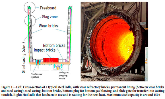
In the steel industry ladles are frequently used to keep, process, or transport steel. Ladles are designed to typically hold metal masses ranging from 80 to 300 t (Figure 1). The melt typically consists of high-temperature liquid steel and some slag, which when interacting with the inner wall of the ladle will harm the wall integrity and cause significant wear. In order to reduce the wear, temperature-resistant and chemically resistant refractory bricks are applied to build an inner barrier, typically three layers of wear bricks (inner lining) which should last for a long time in contact with the liquid steel, and at the same time protect the ladle from showing hot areas. In this paper we address the inner lining erosion of a ladle utilized in secondary metallurgy (SM) at a Sidenor plant. Sidenor is the largest manufacturer of special steel long product in Spain, and is an important supplier of calibrated products in Europe.

 

 

During SM many processes may be going on. The SM ladles have a porous plug installed at the bottom. Gas (Ar or N₂) is injected through the plug to induce liquid steel stirring. The rising flow of the liquid steel promotes the transfer of inclusions from the steel to the slag, and homogenizes the temperature and chemical composition.

The main objective of SM is to obtain the correct chemical composition and appropriate temperature for the casting process. In addition, there are several important processes which must be complete during SM, for example the removal of inclusions and gases. In order to attain these objectives, Sidenor has a SM mill consisting of two ladle furnaces (LFs) and a vacuum degasser (VD). Each of the LFs has three electrodes for heating the slag, steel, and ferro-additions. The ladle contains steel and slag for the whole production process, from EAF tapping to the completion of the casting process. The liquid steel in the ladle has a temperature of around 1700 K, and is covered with slag. The slag, which helps to remove impurities from the steel and prevents contact between the steel and atmosphere, has lower density than steel. The slag consists basically of lime and oxides. Slag conditioning can be improved during SM by adding slag-formers such as lime and fluorspar. In order to handle the liquid steel and slag at such high temperature, the ladle is built with a strong outer steel shell lined inside is with layers of insulating refractory ceramic materials. The most important properties of the refractory lining are:

> Ability to withstand high temperatures

> Favourable thermal properties

> High resistance to erosion by liquid steel and slag.

The inner layer of refractory bricks, which is in contact with the liquid steel, is eroded by the interaction with the hot metal and the slag. Each heat erodes the refractory bricks, and after several heats, they are so eroded that it is not safe to continue using the ladle. The refractory is visually checked after each heat and depending on its state, it may be used for another heat, put aside for repair, or demolished. In case of repair, the upper bricks of the ladle, which are more eroded due to chemical attack by the slag, are replaced and the ladle is put back into production. Later, based on continuing visual inspection, the ladle may be deemed ready for demolition. In this case, the entire inner lining is removed and the ladle relined with new bricks.

One important goal for Sidenor is to reduce refractory costs by identifying new methods for extending the refractory life. One of the key points is to increase the number of heats without compromising safety. Another important issue is to better understand the mechanism of refractory erosion, in order to improve working practices and so increase ladle lifetime.

Motivation

The main goal of this investigation is to develop a model whose results, in conjunction with operator experience, can indicate whether the ladle can be safely used for another heat. The model should incorporate both historical and current production data.

In addition, the model should provide information about the major factors that contribute to ladle refractory erosion and indicate practises that could be adopted to extend refractory life.

 

Previous work on ladle lining erosion

Several studies have been published dealing with properties of refractory bricks (Mahato, Pratihar, and Behera, 2014; Wang, Glaser, and Sichen, 2015), advising on improvements to produce high-quality bricks. A more general review of MgO-C refractories was given by Kundu and Sarkar (2021). The corrosion-erosion mechanisms have been studied in a few papers (Kasimagwa, Brabie, and Jönsson, 2014; Jansson, 2008; Mattila, Vatanen, and Harkki, 2002; Huang et al., 2013; LMM Group, 2020; Zhu et al., 2018). In the opinion of these authors, the most thorough approach was that of Zhu et al. (2018). Bai et al. (2022) investigated the impact of slag penetration into MgO-C bricks.

In order to predict refractory erosion, temperature, fluid composition, and mass transfer mechanisms must be considered. The heat balance has been studied in some specialized works (Çamdali and Tunç, 2006; Glaser, Görnerup, and Sichen, 2011; Zimmer et al., 2008; Duan et al., 2018; Zhang et al., 2009). The effect of slag composition has been studied in multiple works (Bai et al., 2022; Jansson, 2008; Kasimagwa, Brabie, and Jönsson, 2014; Mattila, Vatanen, and Harkki, 2002; Sarkar, Nash, and Sohn, 2020; Sheshukov et al., 2016; Zhu et al., 2018). A critical step in developing prediction models is the local mass transfer between the lining and slag/metal. This has to date been treated by semiempirical models Bai et al., (2022); Sarkar, Nash, and Sohn, 2020; Wang et al., 2022). Wang et al., (2022) applied 3D computational fluid dynamics (CFD) and their predictions seemed to agree with observations. However, they did not report the diffusivities used in their model, and the underlying erosion-corrosion models were empirical and tuned to the data. It was found that these tuning factors would depend on the operating conditions.

In industry, refractory wear is known to be a result of (i) thermal stresses, resulting in thermal spalling, (ii) dissolution of the refractory bricks into the slag/metal, and (iii) dissolution of the binder materials into the slag/metal. Moreover, mechanical stresses imposed on the refractory during cleaning operations will impact on erosion and lifetime. Phenomena such as spalling due to hydration of the bricks are also involved (Wanhao Refractory, 2023).

The impact of thermal stresses will be most severe at the bottom of the ladle when hot steel meets colder refractory. As the velocity of the metal at the moment of impact is high, this is where the maximum thermal stresses are expected. The colder the ladle wall is when it meets hot steel at high speed, the greater the risk of crack formation.

It must be noted that the time between heats has a significant effect on thermal spalling. The temperature distribution in the ladle refractory wall at the time of filling is an important parameter that can be predicted using the model to be presented. However, the addition of a heating burner at the ladle waiting station is not included for now. Instead, we simulate a reduced waiting time to mimic the effects of using a burner to maintain refractory temperature.

 

The pragmatism-based approach to a model for ladle lining erosion

In previous publications, the authors defined a methodology 'Pragmatism in industrial modelling' (Johansen and Ringdalen, 2018; Johansen et al., 2017; Zoric et al., 2015), which is especially suited for developing fast and sufficiently accurate industrial models. In a twin paper (Johansen et al., 2023) the authors have outlined the methodology that was applied in this work and the learnings that may be exploited in future projects. Here the details of the physics-based model are explained.

The objective of the model is to be able to advise or support operators in assessing if it is safe to use the ladle for another heat. In such an application, the erosion state of the refractory must be updated from heat to heat and a simulation for a subsequent virtual heat performed. The virtual heat should contain as much information as possible about the next heat. The result of such a simulation and visual or optical inspection of the lining would then lay the foundation for the final assessment.

 

Model simplifications and assumptions

The pragmatic model must be fast as we wish to simulate a transient ladle operation, lasting about two hours, in less than a minute. This is critical as we wish to simulate all ladle operations within a year in a few hours in order for the results to be applied directly in production, to carry out tuning, or perform a parameter sensitivity analysis.

Figure 2 gives some ideas about the phenomena involved. The heating elements (electrodes) can be submerged in the slag, or work from above. They produce electric arcs that heat the liquid steel. The flow of the slag and liquid steel is not only a function of the gas flow rate applied for blowing, but is also influenced by several factors such as the mass of steel and slag, vacuum pressure, and the thermophysical properties of the fluids.

 

 

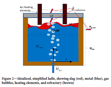
The ladles are 3D objects, but due to speed requirements some overall model simplifications were done:

i. The model is 2D (cylinder-symmetrical) with the porous bottom plug placed in the centre. As a consequence, we assume that the gas/steel/slag flows can be regarded as rotationally symmetric

ii. The stirring gas is inert (only provides mixing)

iii. In the sidewalls only the radial heat balance is included

iv. In the bottom only vertical heat balance is included

v. The solubility of MgO in the slag and of C in the steel are assumed constant

vi. The metal and the slag phases are stratified and are assumed to be internally perfectly mixed. The phases exchange mass and energy with each other and the refractory

vii. Above the slag energy is exchanged by radiation only

viii. Refractory erosion due to thermomechanical stresses is not considered.

 

Volumes and mass balances

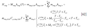
As the model will compute situations with different amounts of steel and slag in the ladle, we have to take into account all these possible situations. The total volume of the slag and metal is represented by

Accordingly, the mass of liquids inside the ladle is:

In our first approach, we neglect the volumes of the protruding impact element at the bottom and the volumes modified by eroded bricks. In this case, the metal-slag interface is positioned at height

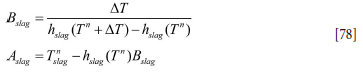
and the thickness of the slag layer is:

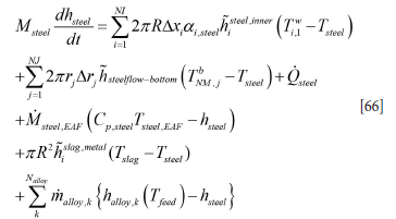
The mass balance for the ladle must also be respected. That is, for the slag

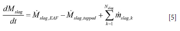
Here M_slag,EAF and M_steel,EAF are the transient mass flow rates of slag and steel coming into the ladle during tapping from the EAF. mslag,k is the mass flow rate of added slag former of type k. Typically a slag former of type k, total mass m_slag,k, can be assumed to be added during one numerical time step, between time tⁿ and tⁿ⁺¹, such that

For the metal we have:

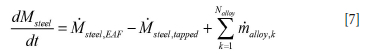
M_slag,tapped and M_steel,tapped are the transient mass flow rates of slag and steel tapped out of the ladle. Similarly, m_alloy,k is the mass flow rate of added alloy of type k. As for the slag, an alloy of type k, total mass m_alloy,k, can be assumed to be added during one numerical time step between tⁿ and tⁿ⁺¹, such that

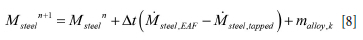
Based on Equations [5]-[8], the phase densities, the purge gas fractions present in each phase, and corrections for the eroded ladle radius, we can compute the transient interface position for the metal and slag. This is critical input to the thermal and erosion models.

 

Thermal models

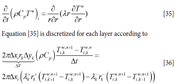
A quasi-2D thermal model for the complete refractory lining and outer steel shell is outlined in Appendix A. Thermal modelling. Both the sidewall and the bottom are included. The model is referred to as quasi2-D as vertical heat transport between horizontal brick layers is assumed to be insignificant compared to heat exchange with metal, slag, and radiation and is ignored. The steel shell exchanges energy with the surroundings while the wetted inner refractory layer exchanges energy with the liquid steel and slag. Nonwetted refractory elements are exchanging energy with the top slag-metal surface, and internally, both by radiation. Enthalpy-based conservation models for steel and slag are developed, as detailed in Appendix A. In general, appropriate boundary conditions are developed and outlined in the appendixes.

Discrete equations for the slag and metal energy

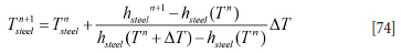
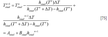
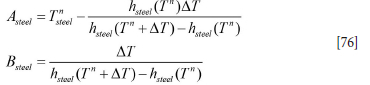
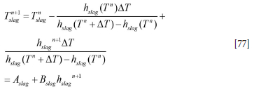
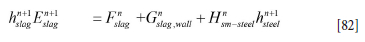
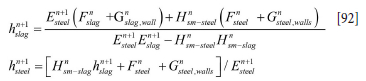
The coupled discrete equations for slag and metal enthalpy (see Equations [64] and [66], Appendix A) can be solved analytically, provided the inner refractory wall temperatures are known. First, we need to establish the relationship between temperatures and enthalpies. This is elaborated in Appendix C. Temperature-enthalpy relationships. As seen from Appendix D. Discrete equations for the slag-metal heat balance, explicit expressions for the slag and metal enthalpies are given by Equation [92]. Temperatures are then computed by Equations [75] and [77].

 

Erosion model

The erosion is primarily a result of dissolution and mass transfer from the refractory into the metal and slag. The erosion mechanism considered is mass loss of refractory to the liquid by dissolution. In addition, we have mass losses due to thermal stresses. These may be addressed in a machine learning model, which may exploit the predicted difference between refractory temperature and that of the incoming steel temperature.

Refractory loss in the steel wetted region

During periods of considerable agitation of the metal and slag (bubble-driven convection, natural convection, electromagnetic stirring) the carbon binder of the MgO-C refractory may be dissolved into the steel. The mass flux of carbon into the steel is locally given by:

Here a_C is the volume fraction of the refractory that is occupied by carbon, D_C is the diffusivity of carbon in steel, and xc is the mass fraction of carbon in the steel.

By introducing the concept of a mass transfer coefficient, we may write Equation [9] as

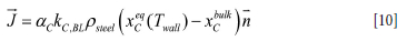
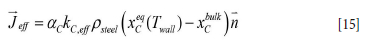
Here kc,BL is the mass transfer coefficient for the liquid side boundary layer and xc^eq (T_wall) is the solubility of C in the steel

with its actual composition, and where T_wall is the temperature at the inner ladle wall. The temperature is controlled by the steel temperature and the temperature in the refractory brick. As the thermal conductivities of the liquid steel and the wear refractory are of the same order of magnitude (see Table I), the wall temperature will depend on both steel and refractory temperature.

For forced convection we may use the mass transfer coefficient suggested by Scalo, Piomelli, and, Boegman (2012) and Shaw and Hanratty (1977), stating that the mass transfer coefficient for Schmidt number Sc > 20 can be approximated by

Values for the shear velocities typically range from zero to 0.1 m/s.

From Equations [10] and [11] we learn that erosion of the steel-wetted ladle wall will increase with increasing gas-stirring flow rate, and temperature (increased C solubility and diffusivity, decreased viscosity).

Mass transfer resistance at the interface between MgO-C and steel

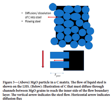
At the inner surface of the MgO-C bricks the C in the C-continuous domains (graphite and carbon contributions from binder) (Zhang, Marriott, and Lee, 2001) will dissolve into the steel while MgO may be considered as inert. A schematic is provided in Figure 3. As the carbon (from carbon-dominated areas) is dissolved into the steel, the average transport length s ^pore will stabilize at around a typical MgO particle radius. If the MgO particles are small the convection inside the pore space can be neglected. In this case the transport in the pore space may be represented by pure diffusion. In that case we can write:

 

 

 

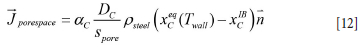
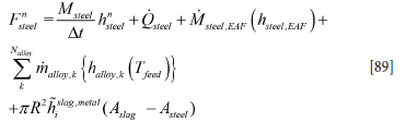
Here x_C^1B is the mass fraction of C at the wall, defined at the outer surface made up if the MgO particles protrude out of the C matrix. In this case the mass flows through the inner and outer layers must match, giving:

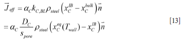
and where the mass transfer coefficient is given by

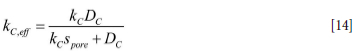
The effective mass transport of C from the MgO-C brick to the steel is then

Refractory loss in the slag-wetted region

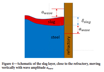
The slag is collected in a relatively thin layer at the surface of the molten bath . Due to the bubble plume, caused by the stirring gas, the slag will be pushed towards the refractory wall. As the bubble plume is asymmetrical, the slag thickness close to the refractory wall will vary along the ladle perimeter. We neglect these complexities and assume complete radial symmetry. The thickness δ_slag of the slag layer that contacts the refractory can be estimated by:

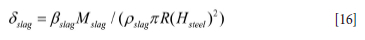
The slag layer will move vertically, driven by waves generated by the bubble plume, as illustrated in Figure 4. The slag layer has thickness δ_slag and wave amplitude a_wave^.

 

 

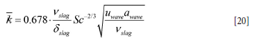
The mass transfer from the wall to the slag layer can be analysed by assuming a developing boundary layer. According to Schlichting (1979) the mass transfer along a developing boundary layer can be expressed as

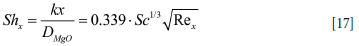
where k is the mass transfer coefficient and x is the distance along the developing boundary layer.

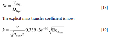
D_MgO is the diffusivity of MgO into the slag, and is related to the Schmidt number by

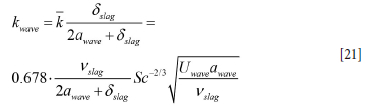
By averaging the mass transfer coefficient k in Equation [19] over the thickness of the slag layer we obtain

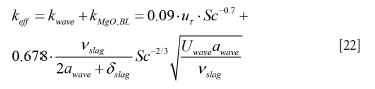
The wave velocity U_wave is now estimated by Equation [108] (Appendix E), and the swept distance (amplitude) a_wave can be represented by l_w in Equation [107]. It is possible to represent the distribution of mass transfer by a probability distribution. However, as a first approximation we assume that the wave-induced mass transfer applies to a region that extends over the thickness of the slag layer and a region that extends a_wave both above and below the slag layer. In this case we may estimate the mass transport to the slag to be given over height 2 a_wave, + δ_slag, and where the average mass transfer coefficient for this layer is

In addition to the explicit wave contribution to mass transfer, the impact of the bubble-driven flow (slag version of Equation [11]) must be added:

Overall refractory loss model

We will track both the MgO and C components of the refractory. We may note that bottom erosion is not included in the model for now. The bottom is included due to its impact on the thermal balance (heat storage).

It is assumed that when C is dissolved from the bricks in the steel region a corresponding amount of MgO is released and will end up in the slag. It is also assumed that the density of the bricks is related to C and the corresponding MgO volume fractions (a_C, a_MgO) and phase densities (p_C, p_mgo) by

where a_C + a_MgO = 1. The MgO mass loss, M_MgO, from a brick element during time dt, eroding a slice of thickness l, is

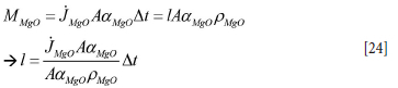
Here A is the total area, and A_aMgO is the partial area where MgO is contacting slag.

The corresponding loss of C due to loss of MgO is then

From Equations [24] and [25] we find that in the slag region the carbon flux out of the refractory wall is given by

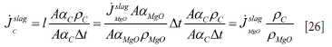
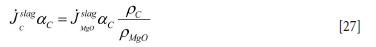
According to Equation [26] the volume flows of the carbon and steel are equal. However, the surface areas are different due to the actual volume fractions. The mass flow of carbon, per unit surface area, to the liquid in the slag region is then

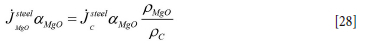
Similarly, the loss of MgO in the steel region due to carbon dissolution is

Carbon balance

The carbon is lost from the refractory by two mechanisms, depending on whether we are consodering the steel-wetted or slag-wetted zone.

The summation is over all the vertical refractory bricks. Here a_i,steel is the local steel fraction (which varies with height in the ladle) and a_C is the carbon fraction in the refractory brick. Ai = 2ϖR∆x_i is the local wall area.

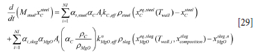
MgO balance

The MgO is lost from the refractory in a similar way to the two mechanisms above.

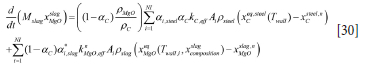
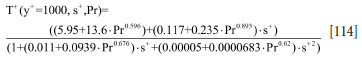
Here a_C is the volume fraction of carbon in the brick, while (1-_aC) is the MgO fraction. a_*i,slag is the wave-enhanced slag fraction, being in contact with the lining. As a first approach for a_*i,slag we use a_*i,slag = 0.25_ai-i,slag + 0.5_ai,slag + 0.25_ai-1,slag.

The left-hand terms are split and the effect of total mass change entered into the models. In the case of the slag we have:

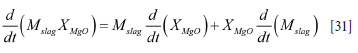
where the mass balance was given by Equation [5]. According to these equations we may write Equation [30] as

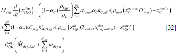
where it is assumed that there is no MgO in the slag tapped from the EAF.

Similarly, the mass balance for carbon becomes

The solubility of MgO in the slag is given as (see acknowledgements) by

Here T is the temperature in degees Celcius. As the slag composition is not known we use a temperature dependency which is approximate for 50 wt%CaO, 10 wt%SiO2, 2.5% FeO, and the balance Al2O3.

 

Developing sub-models - a multi-scale approach

In the present approach we used CFD simulations (Johansen and Boysan, 1988) to obtain the shear stresses along the wall of the ladle. Based on a set of CFD simulations a fitted curve of the vertical shear stress distribution was provided as input for the both the thermal and erosion models (see Appendix B. Wall shear stress model). We did not include the effects of the slag. Using dynamic simulations with slag present more details could be added, and based on curve fitting or lookup tables, the data could be plugged into the model. This would have improved the accuracy.

FACT SAGE calculations were performed for the solubility of MgO in the slag (see Acknowledgements). At the present time it was not possible to use this detailed information as we have no information of the composition of the slag arriving at the ladle from the EAF. Based on this it was possible to close the model equations and realize the models.

 

Software

The model was coded in python 3, using libraries numpy, pandas, math, pickle, and scipy, and we used matplotlib and vtk for plotting and visualization. The basic version of the model is available on github.com, at https://github.com/SINTEF/refractorywear. The model is licensed under the open source MIT license (https://opensource.org/licenses/MIT).

 

Tuning the model

Tables I-III lists the physical and thermodynamic data that was used.

Unfortunately, detailed geometrical data and process data cannot be given due to company confidentiality. In order to apply the model to single heats, operational data from Sidenor was read. The static data included steel mass, time with steel in the ladle, temperature of the steel before leaving the EAF, and cyclic data for vacuum pressure, heating power, measured steel temperatures, gas flow rates, and mass and composition of additions, all versus time. The simulation was initiated at the time when the ladle was filled with liquid steel from the EAF and run for 2 hours. Once the casting process is finished, the ladle is considered to be empty, but still losing heat.

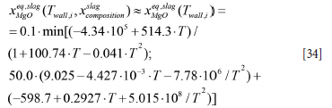
As there is no data on the initial slag mass or composition, it was not possible to incorporate changes in slag composition in the model. The initial slag mass was therefore assumed to be always 500 kg. Another consequence was that we had to assume constant solubilities of C in steel and MgO fraction in the slag. As a result, the solubility of MgO in the slag depends only on temperature (see Equation [34]. Furthermore, all additions were assumed to contribute to the slag. This is acceptable if the alloy additions are of same order of, or smaller than, the pure slag contribution. However, for special steels, addition levels are significant and the model should be updated such that additions are transferred to the metal.

Different additions have different thermodynamic properties, such as melting temperature and melting enthalpy. As this information was largely unknown, we used the same melting temperature and heat of melting for all additions.

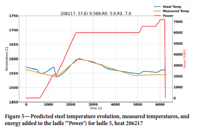
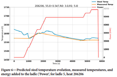
First, we tuned the steel temperature as a good thermal prediction was a prerequisite for the erosion model. At the beginning of each heat it was found that the initial temperature in many cases was a leftover from the previous heat. We therefore decided to use the temperature measured in the EAF, decreasing this by 50 K due to heat loss during tapping. For heats where the initial temperature was unavailable or resulted in large temperature residuals, the initial temperature was corrected in an iterative manner until the residual for average relative temperature was below 20 K. The residual was computed from all measured values except the first, which was not reliable. In both Figure 5 and Figure 6 we see successful simulations, showing zero-order residuals of 5 K and 3 K, respectively. The first-order residuals (RMSE) are similarly 7 K and 5 K. In both cases the initial temperature was optimized, but for heat 206217 the 'measured' initial steel temperature was quite close to the optimized initial temperature. To obtain these results, the thermal efficiency of the heater was reduced to 85% and the thermal conductivity of the refractory bricks and insulation was increased significantly (see Tables I and III).

 

 

 

 

In the second step, the erosion model was tuned. We decided to work with constant solubilities of C in steel (soluble mass fraction was set to 0.1), while the MgO solubility in the slag is based on a fixed slag composition and only varies with temperature (see Table II). As we decided to keep the solubility of C in the steel constant, the only tuning that was possible is the pore diffusion length s _pore (see Equation [12] and Figure 3).

This tuning was done as follows:

i) Start with simulating the preheating of the ladle

ii) Look up the heat ID, then read operational data for the heat and simulate temperature and erosion

iii) Based on the erosion data, reduce the radial cell sizes for the three inner bricks (wear bricks)

iv) Account for the thermal history of the ladle until next heat

v) Repeat step (ii) for the next use of the specific ladle (next heat in campaign, and where the campaign number is unique for the wear lining, from relining until demolition), and then accumulate the erosion of the bricks

vi) If the ladle was taken out for repair of some bricks, the repaired bricks are also repaired in the model. After repair the temperature is again initialized

vii) Repeat step (v) until the ladle is taken out for lining demolition. At this time the predicted erosion profiles are saved and compared to data from the demolition.

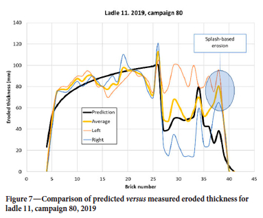
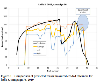
In the demolition data, the ladle is segmented in two halves, where 'Left' is close to the porous plug while 'Right' is away from the plug. In addition, the brick with the most erosion in each half is registered. In this way, a maximum erosion is recorded and the average value for each brick row is not known. However, the 2D model can only be compared with the average of the two and should have some underprediction due to the above observation. For the selected tuning factor s _pore we see that the prediction in Figure 7 is good, both qualitatively and quantitatively. The shape of the erosion in the steel region, below the slag line, is typical for all ladles and campaigns. We note that for bricks 36-40 the erosion level is quite high. This is above the liquid steel level and is a result of metal splashing, causing thermomechanical cracking, and disintegration due to the vacuum treatment (Jansson, 2008). In Figure 8 we see the prediction from a campaign where the erosion in the steel section (bricks 10-25) is underpredicted. Note that in this case, brick numbers below 9 were not measured. The underprediction could be a result of the different steel qualities treated in this specific campaign, or because for some reason the variation along the perimeter, at each brick layer, is larger than usual. As we have no data on the erosion from heat to heat, we cannot tell if this happened during specific heats in the campaign. Another interesting feature, seen in both Figure 7 and Figure 8, is the pronounced dip of erosion around brick 16 and 17. This may be a result of the addition of alloying materials when the ladle is approximately 1/3 full. Alloying elements and slag may stick to the colder wall long enough to protect the lining somewhat.

 

 

 

 

Model performance against Sidenor operational data

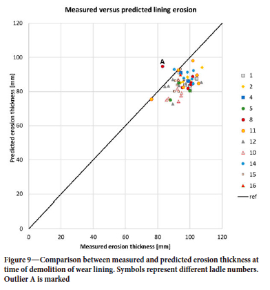
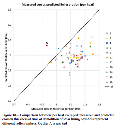
The model was run with all available Sidenor data for 2019. The production campaigns that started in 2018, or ended in 2020, were omitted from the current data-set as those campaigns were not complete. Altogether, we analysed 5216 heats, involving 11 different ladles and 61 campaigns. Averaged erosion over bricks 5-25 is compared in Figure 9. An outlier (ladle 8, campaign 76), marked A, is seen, where the details were already shown in Figure 8. We compare the average erosion per heat in Figure 10, as distributed over the number of heats in each campaign. The model predicts a variation of ±12%, while the data has a variation of ±18%. The outlier A from Figure 9 is clearly seen.

 

 

 

 

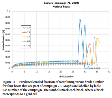
Figures 7 and 8 show a peak in erosion close to the surface of the steel where the slag is located (around brick 35). The steel mass in the ladle varies from heat to heat, but in cases when the reported mass is low this may be due to operation challenges during casting. Therefore, the minimum steel mass is set to 110 t. This introduces another uncertainty in the predictions. Now, it may seem that the erosion does not change much from heat to heat, as indicated from Figure 10. We see in Figure 11 that the predictions show significant difference in amount eroded, and erosion pattern, from heat to heat. Around brick 25 (steel-wetted region) the erosion for use number 17 is around twice as high as for use 69. This difference is mainly due to temperature, time with vacuum, gas flow rates, and operational times. However, when averaged over a complete campaign, these variations are significantly reduced.

 

 

Discussion

The model predicts a smooth increase in erosion rate from the bottom towards the slag. This is in very good agreement with some of the measured erosion profiles. Figure 7 shows one example. This is a result of the bubble-driven flow, enhanced by vacuum, the transport processes in the brick (represented by spore, or s _pore), and in the flow boundary layer, as well as the solubility of carbon in the steel. We used an artificially high value for the saturated carbon mass fraction (X^eq_C = 0.1). However, similar results to those shown here may be obtained by another combination of s _pore and X^eq_C.

We see above that the model performs quite well. At the same time, there is room for improvements. The most obvious improvements are:

i) Modelling of the slag composition and adding the solubility of MgO in the slag as a function of composition. However, this requires knowledge of the composition of the slag tapped from the EAF.

ii) Separating additions into slag formers and alloying elements, and updating the enthalpy-temperature relationships to represent the true compositions of slag and metal.

iii) Empirical slag temperature is needed to calibrate and validate the slag temperature predictions.

iv) Including the solubility of carbon in the steel. Data for the steel composition is available but the carbon solubility for different compositions must also be available.

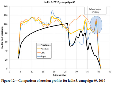
Some features seen in the data, such as shown in Figure 12, cannot be reproduced by the model. The very high observed erosion rates close to the bottom cannot be explained with the available information about the operation. It is possible that gas purging was done with a very low steel level and containing slag. Such issues can be regarded as abnormal operations. Other possibilities are excessive mass loss during ladle cleaning, or that the lining brick quality was not consistent for a period.

 

 

Conclusions and recommendations

The presented model predicts the evolution of lining erosion fairly well. Much better agreement between model and data is hard to obtain due to uncertainties in operational data, physical data, and measurements. The model is primarily predicting lining erosion based on hydrodynamics and solution of lining elements in steel and slag. The contribution from thermomechanical cracking (thermal spalling) of the lining is not included in the model. However, the model predicts lining temperatures at the time metal is tapped into the ladle. This information can in the future be used to assess thermomechanical brick degradation. As this effect was not included, the model was tuned to predict less erosion than what is observed. Similarly, the lining degradation above the melt, which is particularly pronounced during vacuum treatment, was not included in the model. However, a hole in the lining this far up on the ladle wall has far less serious consequences than holes deep below the steel surface.

Model predictions, as we have presented, will provide important support for the ladle operator when deciding if the ladle can be used for another heat. The model shows how the variation in steel level between heats impacts erosion. If all the heats were run with the same volume of steel this would have an adverse impact on lining lifetime. On the other hand, the refractory life may be extended by running scheduled amounts of steel in the heats. When the operator is unsure about the ladle conditions, and based on previous experience from running the model, the model prediction will help the operator to make an appropriate decision.

Finally, it must be acknowledged that the heart of the model is based on complex multiphase 2D CFD simulations that provided critical information about the distribution of shear stresses, and resulted in distributed heat transfer and mass transfer coefficients.

The source code is available from https://github.com/SINTEF/refractorywear

 

Acknowledgements

We thank Dr Kai Tang, SINTEF Industry, for his assistance with the FactSage calculations of MgO solubility in slag. The simplified MgO solubility versus temperature was based on this work.

This research was funded by the H2020 COGNITWIN project, which has received funding from the European Union's Horizon 2020 research and innovation programme under grant agreement No. 870130.

 

CRediT author statement

STJ: Conceptualization, methodology, writing - original draft preparation ; BTL: Software, data curation, validation, visualization, writing - reviewing and editing; TRD: Resources, investigation, writing- reviewing and editing.

 

Nomenclature

A area [m²]

p pressure [Pa], or [bar]

V volume [m³]

M mass [kg]

D diffusivity [m²/s]

k mass transfer coefficient [m/s]

J mass flux [kg/m²s]

Nu Nusselt number

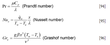
Gr Grashof number

Pr Prandtl number

Ra Rayleigh number

m_alloy mass flow of additions to the ladle during alloying and refining [kg/s]

M mass flow [kg/s]

Sc Schmidt number

s _pore pore diffusion length [m], also denoted s_pore, with ref. to Figure 3

u_t wall shear velocity [m/s]

U_wave wave-induced velocity [m/s] (Equation [108])

a volume fraction

d_slag slag layer thickness [m]

a_wave wave amplitude [m]

β thermal expansion factor [1/K]

ε thermal emissivity [#]

p specific density [kg/m³]

μ fluid viscosity [kg/ms]

v fluid kinematic viscosity [m²/s]

λ thermal conductivity [W/mK]

σ Stefan-Boltzmann coefficient (5.67e-8 W /m²K⁴)

t_w wall shear stress [Pa]

∆h specific heat of melting [kJ/kg]

∆t numerical time step [s]

∆T change in temperature between two time steps: AT = Tⁿ⁺¹ - Tⁿ

∆x, ∆y grid spacings in axial and radial directions [m]

Ψ expression given by Equation [58]

C_p specific heat capacity [J/kg K]

h specific enthalpy [kJ/kg]

h heat transfer coefficient [W/m²K]

H height or distance [m]

H_steel total enthalpy of steel [kJ]

H_slag total enthalpy of slag [kJ]

r radial position [m]

R ladle inner radius [m]

T temperature [K]

x mass fraction, subscripts representing carbon (C) or MgO

Q gas volume flow rate [normal l/min]

q heat flux [W/m²]

Q heat flow [W]

 

Superscripts

eq thermodynamic equilibrium

EAF electric arc furnace

EXT external

IB inner boundary layer

 

References

Ashrafian, A. and Johansen, S.T. 2007. Wall boundary conditions for rough walls. Progress in Computational Fluid Dynamics, vol. 7, no. 2. pp. 230-236. https://doi.org/10.1504/PCFD.2007.013015        [ Links ]

Bai, R., Liu, S., Mao, F., Zhang, Y., Yang, X., and He, Z. 2022. Wetting and corrosion behavior between magnesia-carbon refractory and converter slags with different MgO contents. Journalof Iron and Steel Research International, vol. 29. pp. 1073-1079. https://doi.org/10.1007/s42243-021-00695-y        [ Links ]

Çamdali, Ü. and Tunc, M. 2006. Steady state heat transfer of ladle furnace during steel production process. Journal of Iron and Steel Research International, vol. 13. pp. 18-20. https://doi.org/10.1016/S1006-706X(06)60054-X        [ Links ]

Ceotto, D. 2013. Thermal diffusivity, viscosity and prandtl number for molten iron and low carbon steel. High Temperature, vol. 51, no. 1. pp. 131-134. https://doi.org/10.1134/S0018151X13010045        [ Links ]

Churchill, S.W. and Chu, H.H.S. 1975. Correlating equations for laminar and turbulent free convection from a vertical plate. International Journalof Heat and Mass Transfer, vol. 18. pp. 1323-1329.         [ Links ]

Cloete, S.W.P. 2008. A mathematical modelling study of fluid flow and mixing in gas stirred ladles. MSc thesis). Stellenbosch University, South Africa.         [ Links ]

Duan, H., Zhang, L., Thomas, B.G., and Conejo, A.N. 2018. Fluid flow, dissolution, and mixing phenomena in argon-stirred steel ladles. Metallurgical and and Materials Transactions B, vol. 49. pp. 2722-2743. https://doi.org/10.1007/s11663-018-1350-4        [ Links ]

Ede, A.J. 1967. Advances in free convection. Advances in Heat Transfer. Hartnett, J.P. and Irvine, T.F. (eds). Elsevier. pp. 1-64. https://doi.org/10.1016/S0065-2717(08)70272-7        [ Links ]

Glaser, B., Görnerup, M., and Sichen, D. 2011. Fluid flow and heat transfer in the ladle during teeming. Steel Research International, vol. 82. pp. 827-835. https://doi.org/10.1002/srin.201000270        [ Links ]

Goodman, S. 1957. Radiant-heat transfer between nongray parallel plates. Journal of Research of the National Bureau of Standards, vol. 58, no. 1. pp. 37-40. https://doi.org/10.6028/jres.058.006        [ Links ]

Hiratsuka, A., Tsujino, R., Sasaki, Y., Nishihara, K., and Iguchi, M. 2007. Prediction of the period of swirl motion appearing in gas injection processes at high temperatures. Journal of High Temperature Society, vol. 33. pp. 169-172. https://doi.org/10.7791/jhts.33.169        [ Links ]

Huang, A., Gu, H., Zhang, M., Wang, N., Wang, T., and Zou, Y. 2013. Mathematical modeling on erosion characteristics of refining ladle lining with application of purging plug. Metallurgical and Materiaks Transactions B, vol. 44. pp. 744-749. https://doi.org/10.1007/s11663-013-9805-0        [ Links ]

Huang, A., Harmuth, H., Doletschek, M., Vollmann, S., and Feng, X. 2015. Toward CFD modeling of slag entrainment in gas stirred ladles. Steel Research International, vol. 86. pp. 1447-1454. https://doi.org/10.1002/srin.201400373        [ Links ]

Jansson, S. 2008. A study on the influence of steel, slag or gas on refractory reactions. Doctoral thesis, Department of Material Science and Engineering, Royal Institute of Technology, Stockholm. http://www.diva-portal.org/smash/get/diva2:13829/FULLTEXT01.pdf        [ Links ]

Johansen, S.T. and Boysan, F. 1988. Fluid dynamics in bubble stirred ladles: Part II. Mathematical modeling. Metallurgical Transactions B, vol. 19. pp. 755-764.         [ Links ]

Johansen, S.T., Lovfall, B.T., Rodriguez Duran, T., and Zoric, J. 2024. Pragmatism in industrial modelling: An application to ladle lifetime in the steel industry. Journal of the Southern African Institute of Mining and Metallurgy, vol. 124, no. 3. pp. 111-122.         [ Links ]

Johansen, S.T. and Ringdalen, E. 2018. Reduced metal loss to slag in HC FeCr production - by redesign based on mathematical modelling. Proceedings of Furnace Tapping 2018, Kruger National Park, South Africa, 14-17 October 2018. Steenkamp, J.D. and Cowey, A. (eds). Symposium Series S98. Southern African Institute of Mining and Metallurgy, Johannesburg. pp. 29-38.         [ Links ]

Johansen, S.T., Meese, E.A., Zoric, J., Islam, A., and Martins, D.W. 2017. On pragmatism in industrial modeling Part III: Application to operational drilling. Progress in Applied CFD, CFD2017. Proceedings of the 12th International Conference on Computational Fluid Dynamics in the Oil & Gas, Metallurgical and Process Industries. SINTEF Academic Press, Trondheim, Norway. http://hdl.handle.net/11250/2465068        [ Links ]

Kasimagwa, I., Brabie, v., and Jönsson, P.G. 2014. Slag corrosion of MgO-C refractories during secondary steel refining. Ironmaking & Steelmaking, vol. 41. pp. 121-131. https://doi.org/10.1179/1743281213Y.0000000110        [ Links ]

Kundu, R. and Sarkar, R. 2021. MgO-C refractories: A detailed review of these irreplaceable refractories in steelmaking. International Ceramic Review, vol. 70. pp. 46-55. https://doi.org/10.1007/s42411-021-0457-9        [ Links ]

LMM Group. 2020. Erosion mechanism of magnesia-carbon brick in ladle in slag. https://www.lmmgroupcn.com/erosion-mechanism-of-magnesia-carbon-brick-in-ladle-in-slag/ [accessed 30 November 2022].         [ Links ]

Mahato, S., Pratihar, S.K., and Behera, S.K. 2014. Fabrication and properties of MgO-C refractories improved with expanded graphite. Ceramics International, vol. 40. pp. 16535-16542. https://doi.org/10.1016/j.ceramint.2014.08.007        [ Links ]

Mattila, R.A., Vatanen, J.P., and Harkki, J.J. 2002. Chemical wearing mechanism of refractory materials in a steel ladle slag line. Scandinavian Journal of Metallurgy, vol. 31. pp. 241-245. https://doi.org/10.1034/j.1600-0692.2002.00531.x        [ Links ]

Sarkar, R., Nash, B.P., and Sohn, H.Y. 2020. Interaction of magnesia-carbon refractory with metallic iron under flash ironmaking conditions. Journal of the European Ceramic Society, vol. 40. pp. 529-541. https://doi.org/10.1016/j.jeurceramsoc.2019.09.019        [ Links ]

Scalo, C., Piomelli, U., and Boegman, L. 2012. High-Schmidt-number mass transport mechanisms from a turbulent flow to absorbing sediments. Physics of Fluids, vol. 24. 085103. https://doi.org/10.1063/L4739064        [ Links ]

Schlichting, H. 1979. Boundary Layer Theory. 7th edn. McGraw-Hill, New York.         [ Links ]

Shaw, D.A. and Hanratty, T.J. 1977. Influence of Schmidt number on the fluctuations of turbulent mass transfer to a wall. AIChE Journal, vol. 23. pp. 160-169. https://doi.org/10.1002/aic.690230204        [ Links ]

Sheshuokv, O.Yu., Nekrasov, I.V., Mikheenkov, M.A., EgIazar'yan, D.K., Ovchinnikova, L.A., Kashcheev, I.D., Zemlyanoi, K.G., and Kamenskikh, V.A. 2016. Effect of refining slag phase composition on ladle furnace unit lining life 1. Refractories and Industrial Ceramics, vol. 57. pp. 109-116. https://doi.org/10.1007/s11148-016-9937-2        [ Links ]

Sidenor. Not dated. https://www.sidenor.com/en/f accessed 28 August 2023).         [ Links ]

Wikipedia. 2022. View factor.https://en.wikipedia.org/wiki/View_factor        [ Links ]

Wang, H., Glaser, B., and Sichen, D. 2015. Improvement of resistance of MgO-based refractory to slag penetration by in situ spinel formation. Metallurgical and Materials Transactions B, vol. 46. pp. 749-757. https://doi.org/10.1007/s11663-014-0277-7        [ Links ]

Wang, Q., Jia, S., Qi, F., Li, G., Li, Y., Wang, T., and He, Z. 2020. A CFD study on refractory wear in RH degassing process. ISIJ International, vol. 60. pp. 1938-1947. https://doi.org/10.2355/isijinternational.ISIJINT-2019-768        [ Links ]

Wang, G., Liu, C., Pan, L., He, Z., Li, G., and Wang, G. 2022. Numerical understanding on refractory flow-induced erosion and reaction-induced corrosion patterns in ladle refining process. Metallurgical and Materials Transactions B, vol. 53. pp. 1617-1630. https://doi.org/10.1007/s11663-022-02471-z        [ Links ]

Wanhao Refractory. 2023. 4 effective measures to improve the life of ladle. https://www.linkedin.com/pulse/4-effective-measures-improve-life-ladle-sujiao-zhao-agyfe?trk=article-ssr-frontend-pulse_more-articles_related-content-card [accessed 13 February 2023].         [ Links ]

Warner, C.Y. and Arpaci, VS. 1968. An experimental investigation of turbulent natural convection in air at low pressure along a vertical heated flat plate. International Journal of Heat and Mass Transfer, vol. 11. pp. 397-406. https://doi.org/10.1016/0017-9310(68)90084-7        [ Links ]

Zhang, S., Marriott, N.J., and Lee, WE. 2001. Thermochemistry and microstructures of MgO-C refractories containing various antioxidants. Journal of the European Ceramic Society, vol. 21. pp. 1037-1047. https://doi.org/10.1016/S0955-2219(00)00308-3        [ Links ]

Zhang, S.F., Wen, L.Y., Bai, C.G., Chen, D.F., and Long, Z.J. 2009. Analyses on 3-D gas flow and heat transfer in ladle furnace lid. Applied Mathematical Modelling, vol. 33. pp. 2646-2662. https://doi.org/10.1016/j.apm.2008.08.003        [ Links ]

Zhu, L., Jia, Y., Liu, Z., Zhang, C., Wang, X., and Xiao, P. 2018. Mass-transfer model for steel, slag, and inclusions during ladle-furnace refining. High Temperature Materials and Processes, vol. 37. pp. 665-674. https://doi.org/10.1515/htmp-2017-0011        [ Links ]

Zimmer, A., Lima, Á.N.C., Trommer, R.M., Bragança, S.R., and Bergmann, CP. 2008. Heat transfer in steelmaking ladle. Journal of Iron and Steel Research International, vol. 15. pp. 11-14. https://doi.org/10.1016/S1006-706X(08)60117-X        [ Links ]

Zoric, J., Busch, A., Meese, E.A., Khatibi, M., Time, R.W., Johansen, S.T., and Rabenjafimanantsoa, H.A. 2015. On pragmatism in industrial modeling - Part II: Workflows and associated data and metadata. Proceedings of the 11th International Conference on CFD in the Minerals and Process Industries, Melbourne, Australia, 7-9 December 2015. Solnordal, C.B., Liovic, P., Delaney, G.W., Cummins, S.J., Schwarz, M.P. and Witt, P. J. (eds). 7 pp. http://www.cfd.com.au/cfd_conf15/PDFs/032JOH.pdf        [ Links ]

Zoric, J., Johansen, S.T, Einarsrud, K.E., and Solheim, A. 2015. On pragmatism in industrial modeling. Progress in Applied CFD; Selected Papers from 10th International Conference on Computational Fluid Dynamics in the Oil & Gas, Metallurgical and Process Industries. Volume 1.Sintef Academis Press, Trondheim, Norway. pp. 9-24.         [ Links ]

 

 

Correspondence:
S.T. Johansen
Email: Stein.T.Johansen@sintef.no

Received: 13 Mar. 2023
Revised: 17 Jul. 2023
Accepted: 27 Sep. 2023
Published: March 2024

 

 

Appendix A. Thermal modelling

Ladle sidewall energy model

The ladle sidewall is built with a number of radial layers, as shown in Figure 13. Next, we let the numerical grid, as seen in the figure, represent each vertical layer of wear bricks, and stack multiple layers on top of each other to represent the entire sidewall of the ladle. The colours in Figure 13 represent different properties of the materials. The bottom part of the refractory is built of a stack of discs, which also may be represented by Figure 13, but now rotated 90^o clockwise.

 

 

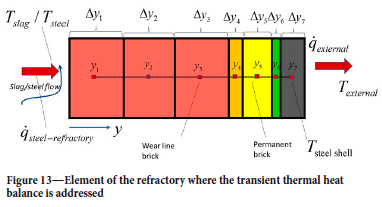
In this manner, the numerical grid for the ladle wall and casing temperature will consist of a single one-dimensional grid (here 7 cells) for the bottom and N one-dimensional grids for the vertical wall (N X 7 cells). For the horizontal and radial heat balance we have

Superscripts + and - represent the value at the positive and negative sides of the cell face. ∆_xi is the vertical height of the grid cell at level i cell while r_k is the radial position index for the cell. We use harmonic averages for the cell face thermal conductivities and λ_k+1 and λ⁺_k

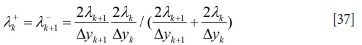
where r_k is defined according to Figure 13:

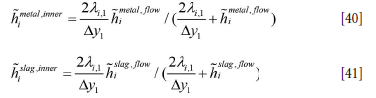
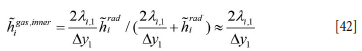
In the cell contacting the hot liquid steel and slag (k = 1) we have

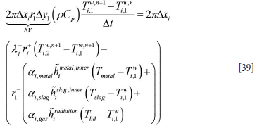
In Equation [39] a_i,metal, a_i,slag, and a_i,gas are the local volume fractions of the phases contacting the element ∆_xi at a given time.

where the external temperature is given by Text. The radiation heat transfer coefficient is given by

and where the wall temperature is further approximated by the temperature in the near wall cell at the previous time step:

For the outer wall at y_Nj = y7 (steel casing) we have:

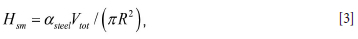
Here the external heat transfer coefficient is estimated by the sum of natural convection and radiation. The convective external heat transfer coefficient h_NC is given by Equation [104] using the properties for air. The dimension used in the convective model should be the half height of the ladle standing straight up. The effective external heat transfer coefficient is then

When the ladle is located inside a cabinet, within a compartment with external walls, the effective heat emissivity in Equation [46] can be multiplied by a factor of 0.5.

It should be noted that the external heat transfer coefficients must be adjusted to the situation the ladle experiences (melt refining, transport to casting station, casting, transport to waiting station, waiting). If the external heat transfer conditions varies between the different events, this must be handled in an appropriate manner such that we can tune the model to get a realistic thermal history for the ladle.

Ladle bottom energy model

The model for the bottom energy is completely analogous to that described above, but now with the discrete equation

Here R is the inner radius of the ladle. For the element close to the liquid steel (we assume that steel flows into the bottom at time = 0.0 s) we have:

For the bottom element (steel shell) we have:

where we estimate

Radiation - Wall temperatures and heat transfer above the slag/metal

Above the liquid phase the refractory will only see the top lid, the other parts of the wall, and the metal surface. We will assume that the top lid is adiabatic, such that no energy is drained out through the lid. We now have to assess radiation transfer between different inner wear bricks and the top surface of the slag/metal. The radiative flux from a surface with emissivity ε_p and temperature T_p is given by

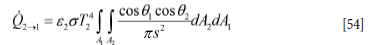
The radiation heat flow from surface elements A₁ to A₂ is given by (Wikipedia, 2022)

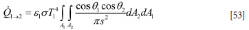
The geometrical configuration is seen in Figure 14.

 

 

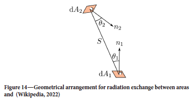
The radiation heat flow from A₂ to A₁ is then

The heat flow between the two surfaces A₁ and A₂ can be given by (Goodman, 1957):

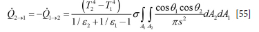
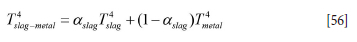
Based on Equations [52]-[55], the surface normal vectors n₁ and n₂, and the vector connecting area elements dA1 and dA2, all radiation heat flows can be computed. These are Q _{W,m ->slag-metal} (from brick number m to slag-metal interface), Q_w,m->ceiling (from brick number m to ceiling), and Q_{slag-metal->ceiling} (from slag-metal interface to ceiling). The direct radiation between bricks is ignored. The radiation from the slag-metal interface must respect that the slag only covers a fraction a_slag of the total free surface area. Hence, the radiation temperature T_s⁴_lag-metal is replaced by:

It is further assumed that the ceiling (ladle lid) is adiabatic and that the slag and metal are well mixed. However, for the refractory bricks the thermal conduction heat flux into the inner wall surface brick and the net radiation flux must balance. The surface temperature of the wall bricks is then given as

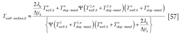
This illustrates the fact that it is surface temperature that communicates radiation and not volume-averaged temperature for the computational cell.

The factor Ψ is given by

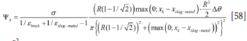
where ∆0 is the horizontal area element (per radian) which exchanges radiation between slag/metal and bricks.

The heat flows may be converted to heat transfer coefficient by rewriting Equation [55] as

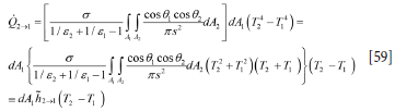
where h_2->1 is the heat transfer coefficient expressed by the bracketed terms in Equation [59] above.

As the lid is adiabatic we have the following condition to fulfil:

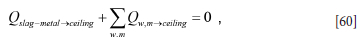
From Equation [60] we compute the ceiling temperature.

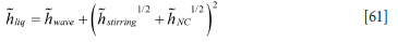
Effective heat transfer coefficient

The effective heat transfer coefficient h_liq in the liquid steel and slag may now be estimated based on three different contributions:

1. The wave induced contribution h_wave, elaborated in Appendix F. Wave-induced heat transfer 2. The heat transfer due to bubble stirring h_stirring, elaborated in Appendix G. Inner wall heat transfer coefficients due to forced convection by bubble stirring

3. The heat transfer due to natural convection h_NC elaborated in Appendix E. Pure natural and effective convection heat transfer:

 

Heat balance for the slag

Due to the melting of additives (slag formers, refining additions, alloying elements) we have selected to represent the energy by the specific enthalpy h.

First, we give the slag enthalpy by a simplified relationship:

Here the enthalpy for the solids is represented by C_p,sT, and for the liquids by C_p,sT₁ + ∆h+C_p,l (T-T₂), where C_p,l is the liquid heat capacity and ∆h is the latent heat of fusion. The temperatures T₁ and T₂ are the temperatures at which the phase transition (melting) starts and is completed, respectively.

The heat balance for the slag is then

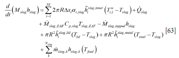
Here a_i,slag is the slag fraction contacting brick number i and varies with time. T_feed is the temperature of the materials at the time of feeding, typically less than 100°C. M_slag,EAF is the time-dependent mass flow of slag from the EAF. h_i^slag,lid is the heat transfer coefficient for slag surface - top lid heat exchange, and h_i^slag,metal is the area-averaged heat transfer coefficient between the metal and slag. Q_slag is the heating power supplied to the slag [W/kg]. All these quantities are in general varying with time.

By subsituting the mass balance (Equation [5]) into Equation [63] we obtain:

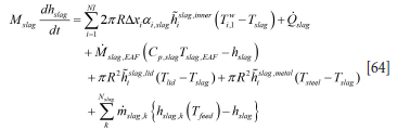
We may note that Equation [64] indicates that the slag components, fed at low temperature T_feed, will lower the enthalpy of the slag as h_slag,k (T_feed) - h_slag < 0.

Heat balance for the metal

As for the slag, the metal enthalpy H_steel can be expressed by the specific enthalpy h_steel:

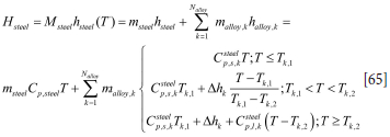
Similarly, for the metal (steel) we have

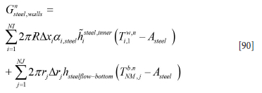
The first right-hand-side sum represents the heat transfer along the vertical ladle wall, while the second summation term represents the heat transfer between steel and the bottom refractory. It is assumed that the bottom heat transfer is zero before steel is received in the ladle.

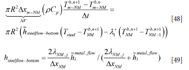
a_i,steel is the metal fraction contacting brick number i and varies with time. M_steel,EAF is the time-dependent mass flow of steel from the EAF. hs_{teelflow-bottom} is the heat transfer coefficient for metal-bottom refractory heat exchange, and h_i^slag,metal is the area-averaged heat transfer coefficient between metal and slag. Q_steel is the heating power supplied directly to the steel [W/kg]. Again, these quantities are in general varying with time.

The heat source and Q_slag are related to the total power Q_tot supplied by the heating electrodes. Q_tot is the power logged at the plant. The heat entering the slag and metal will be lower. We introduce an overall heating efficiency N_eff [0,1] and a heat distribution coefficient N_slag, such that

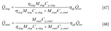
The coefficient N_slag = 1.0 indicates that slag and metal increase in temperature at the same rate. If N_slag = 2.0 the slag temperature increases twice as fast as that of the steel. If N_slag = 0.5 the slag temperature increases at half the rate of the steel. The introduction of the coefficient N_slag allows a more controlled way to distribute heat between the steel and slag.

Solution for the wall energy equations

Based on previous temperatures the radiation flows and fluxes are computed (Equations [52]-[57]). For the radial wall elements the discrete equations [36], [39] and [47] can be written as

Here b^w_i will contain reference to previous slag and metal temperatures, radiation fluxes, and external temperatures. The solution is obtained by inverting the NJ x NJ (here 7 x 7) matrix A_i:

We notice that while the ladle is in steady operation (no filling or tapping) the matrix A_i is fixed. In this case the new wall temperatures are obtained by only updating b^w_i , which depends on values from previous time step, and then repeating the matrix-vector operation in Equation [70]. This allows very fast solution of wall temperatures.

The bottom part of the wall is solved in the same manner.

 

Appendix B. Wall shear stress model

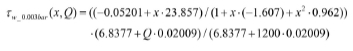
The steady-state flow in the ladle was simulated (Johansen and Boysan, 1988) for the different (500, 600, 800, and 1200 Nl/ min) argon gas flow rates, using a typical steel mass (130 t) and ladle geometry from Sidenor. In addition, the simulations were performed for both atmospheric pressure and 0.003 bar above the melt. The simulated wall stresses were expressed by fitting functions and the effect of pressure was handled by a linear fit between the atmospheric and near-vacuum pressures.

Denote P as pressure in atmospheres (P = 1 bar = 1e5 Pa) , and we have volume flow of argon Q in normal litres per minute (nl/ min), relative heigh x = X/H.

Wall stress data for low pressure (P = 0.003 bar):

Wall stress data for normal pressure (P = 1.000 bar):

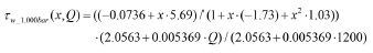
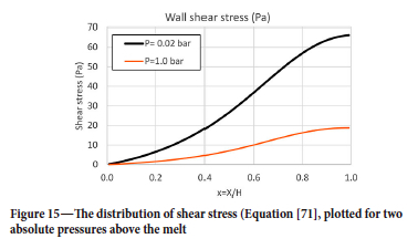
From the two fits above the wall stress distribution, including operating pressure, becomes

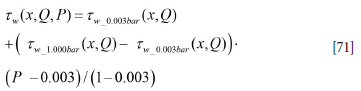
Equation [71] is simply the new model. The result is shown in Figure 15.

 

 

Wall shear velocity u_t now becomes

 

Appendix C. Temperature-enthalpy relationships

As we use both enthalpy and temperature, we establish some critical relationships.

In the case of the steel, we can find the temperature from the enthalpy by a Taylor expansion of the enthalpy function:

According to Equation [73] the temperature is

As we wish to replace the temperatures of the slag and metal with enthalpies, we carry out the following reorganizations:

where

Similarly, for the slag we obtain:

where we have

Based on Equations [73]-[78] we can produce coupled enthalpy equations for the metal-slag-refractory system.

 

Appendix D. Discrete equations for the slag-metal heat balance

Fluid temperatures

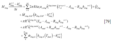
We can now write discrete equations for the slag and steel temperature. We use implicit treatment of the right-hand-side enthalpies. The slag heat balance, given by Equation [64] now reads

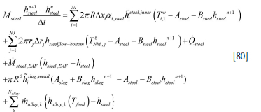
while for the metal (steel) heat balance we have

The discrete equation for the slag can be written in a simplified form:

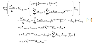
We simplify Equation [81] as

where

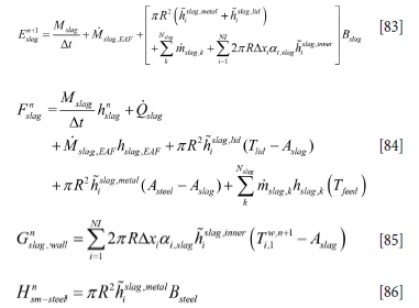
We have here treated the internal wall temperature in an explicit manner in order to be able to separate the set of equations and allow fast computations. The coefficients represented by Equations [83]-[86] have to be updated for every time step.

For the steel phase we may, based on Equation [80], write

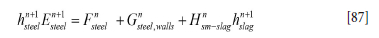
where

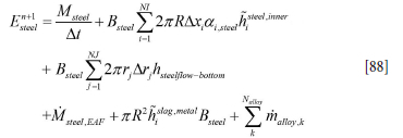
and

and

and where

The solution for Equations [82] and [87] is trivial, giving:

The calculations of temperatures from the enthalpies are given by Equations [75]-[78].

 

Appendix E. Pure natural and effective convection heat transfer

According to Ede (1967) the heat transfer due to pure natural convection can be estimated by:

where:

An average distance x may be estimated by the liquid height

Hsteel, giving x³ = H_steel³,

and

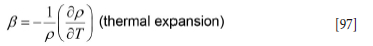
The Churchill-Thelen correlation (Churchill and Chu, 1975) gives:

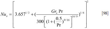
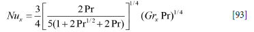
The latter correlation is fine for turbulence controlled natural convection. However, for Ra = GrxPr smaller than 10¹⁰ the model given by Equation [93] is very good. We therefore propose a mixture of the two models with a transition at Ra = GrxPr = 2-10¹⁰.

The assembled model then becomes:

where

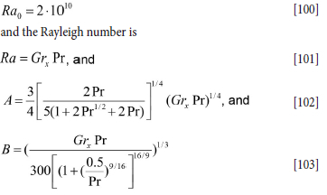
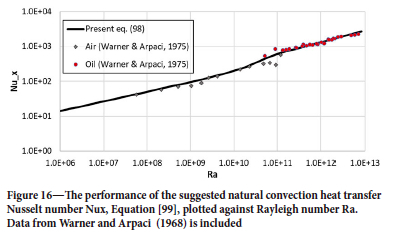
See Figure 16 for comparison with the base correlations. The heat transfer coefficient due to natural convection is now:

 

 

 

Effective heat transfer coefficient

The effective heat transfer coefficient in the liquid steel and slag may now be estimated from

 

Appendix F. Wave-induced heat transfer

The bubble plume impinging on the surface will produce waves at the interface (Cloete, 2008). An empirical correlation for the wave period T_s was produced by Hiratsuka et al. (2007)

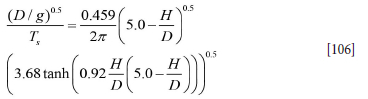
where D is ladle diameter and H is liquid height. The length swept by the wave is l_W, where

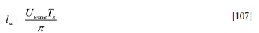
The wave velocity is here based on the turbulent velocities near the wfree surface. From 2D CFD simulations we have curve-fitted the computed turbulent velocities as:

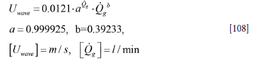
According to Equation [108] the wave velocities Uwave will range between 0.13 and 0.18 m/s for gas flow rates ranging between 500 and 1200 l/min.

According to Blasius:

Over the distance l_w /2 and average velocity u = , the averaged heat transfer coefficient h_Wave* is:

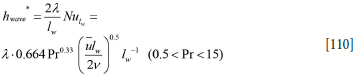
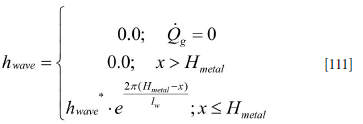
The wave-induced added heat transfer will apply to a region close to the surface. Due to the small thickness of the slag layer, it is proposed that the wave-induced heat transfer applies only to the metal, given by the following relationship:

 

Appendix G. Inner wall heat transfer coefficients due to forced convection by bubble stirring

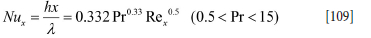
The heat transfer coefficients due to forced convection can be obtained from the definition of the dimensionless flow temperature T⁺:

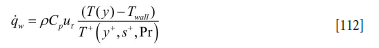
Here q_w is the wall heat flux, u_x is the wall shear velocity, defined by u_t = = yu_t/v is the non-dimensional wall distance, and s+ = su_t/v is the non-dimensional wall roughness.

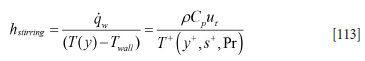
The resulting heat transfer coefficient then becomes

Using a wall function model (Ashrafian and Johansen, 2007) the T⁺ function can be evaluated at a typical bulk fluid wall distance y+= 1000, and for a given hydrodynamic roughness height s+ = s ■ u_t/v), where v is the kinematic viscosity of the steel.