


Services on Demand
Article
 English (pdf)
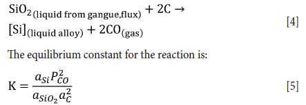
 Article in xml format
 Article references
Indicators

Related links
-
 Cited by Google
 -
 Similars in Google
Share

 Permalink
Journal of the Southern African Institute of Mining and Metallurgy
On-line version ISSN 2411-9717
Print version ISSN 2225-6253
J. S. Afr. Inst. Min. Metall. vol.124 n.2 Johannesburg Feb. 2024
http://dx.doi.org/10.17159/2411-9717/2297/2024
PROFESSIONAL TECHNICAL AND SCIENTIFIC PAPERS
Prediction of silicon content of alloy in ferrochrome smelting using data-driven models
A.V. CherkaevI; M. ErweeI; Q.G. ReynoldsII, III; S. SwanepoelI
ISamancor, South Africa. ORCID: A.V. Cherkaev. http://orcid.org/0000-0002-7637-0732
IIPyrometallurgy Division, Mintek, South Africa
IIIDepartment of Chemical Engineering, Stellenbosch University, South Africa
SYNOPSIS
Ferrochrome (FeCr) is a vital ingredient in stainless steel production and is commonly produced by smelting chromite ores in submerged arc furnaces. Silicon (Si) is a componrnt of the FeCr alloy from the smelting process. Being both a contaminant and an indicator of the state of the process, its content needs to be kept within a narrow range. The complex chemistry of the smelting process and interactions between various factors make Si prediction by fundamental models infeasible. A data-driven approach offers an alternative by formulating the model based on historical data. This paper presents a systematic development of a data-driven model for predicting Si content. The model includes dimensionality reduction, regularized linear regression, and a boosting method to reduce the variability of the linear model residuals. It shows a good performance on testing data (R2 = 0.63). The most significant predictors, as determined by linear model analysis and permutation testing, are previous Si content, carbon and titanium in the alloy, calcium oxide in the slag, resistance between electrodes, and electrode slips. Further analysis using thermodynamic data and models, links these predictors to electrode control and slag chemistry. This analysis lays the foundation for implementing Si content control on a ferrochrome smelter.
Keywords: ferrochrome, silicon content, machine learning, principal component analysis, gradient boosting, mutual information.
Introduction
Ferrochrome (FeCr) is an alloy commonly used as raw material in the production of stainless steel and special steels requiring corrosion and creep resistance. The largest deposits of chromite ore occur in South Africa (Haldar, 2020). Most of the ferrochrome is produced by means of fluxed smelting of chromite ore using quartz and limestone in a submerged arc furnace (SAF). Typically, FeCr produced in this process contains about 50-53% Cr, 4-6% Si, and 6-8% C with the balance being Fe (Gasik, 2013).
The reduction of chromite with carbon in SAFs is quite complex, and has been documented in detail by several authors (Xiao, Yang, and Holappa, 2006; Hayes, 2004; Ringdalen and Eilertsen, 2001; Wedepohl and Barcza, 1983), but the overall reactions can be simplitied as follows:
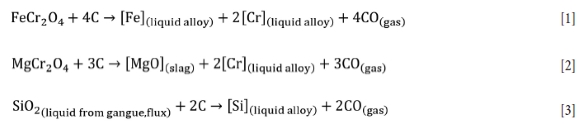
Typically, slag is tapped at temperatures above 1700°C, with an average in-furnace temperature in the order of 1800°C. At these temperatures, the undesirable reduction of SiO2 (Equation [3]) is thermodynamically favourable and directly in competition with the first two chromite reduction reactions. The alloy thus becomes contaminated with Si. Aside from the quality issue, every 1% increase in Si content adds some 45 kWh per ton alloy to the specific energy requirement for smelting (Ringdalen, Rocha, and Figueiredo, 2015). In contrast, a low Si content in the alloy indicates a lack of active carbon for reduction reactions (Urquhart, 1972). It is for these reasons that understanding how to control Si in SAF smelting of chromite is important.
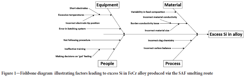
A target Si content in the alloy of no more than 4.5% is desirable as per general customer specifications. The exact mechanisms that can lead to variation of Si in the alloy are quite complex, and beyond the scope of this paper. The reader is referred to the literature for more information on the topic (see Ranganathan et al., 2005; Ranganathan and Godiwalla, 2011; Hockaday and Bisaka, 2010; Geldenhuys, 2013; Erwee, Swanepoel, and Reynolds, 2021). A simplistic summary of these effects in SAF smelting of chromite is given in Figure 1. It is important to note that the diagram does not highlight all the interactions between the different causes; these are alluded to in the literature cited above. Due to the complexity of the process, machine learning methods can offer not only insight into the relative importance of the drivers for Si content of the alloy, but also a possible means of control by way of supporting decisions-made by operators.
Machine learning methods for process monitoring
Machine learning (ML) methods have been applied for process monitoring tasks in various industries for over a decade (McCoy and Auret, 2019) to support decision-making by operators and, where possible, to automate it. At a more technical level, ML models are used for such tasks as data cleaning, missing data imputation, and noise reduction (unsupervised methods that include dimensionality reduction and clustering), and soft sensing and forecasting (supervised methods that include regression and classification). Unsupervised methods are characterized by the absence of the output, or response, variable i.e., the target is unknown. Their aim is to simplify and condense the data. In contrast, supervised methods aim to infer or predict a particular response, e.g., temperature in a reactor, liquid level in a vessel, product composition, etc.
The rest of this subsection describes the process of ML model application to industrial data, starting with the terminology as this is quite specific to the ML field.
Terminology
The data-set used for ML models is a table of entries consisting of M rows and N columns. Each column corresponds to a feature being measured. For example, hearth temperature, current through electrode, type of reductant, etc. A column is referred as a variable. A variable that is aimed to be inferred by an ML model is referred as a target, response, or output variable. Other variables are called predictors or features. The number of columns N determines the dimensionality of the data (target variables are usually excluded from it). Each row of the table corresponds to an individual observation and, thus, the term observation is used to denote a row (James et al., 2017).
Using a probabilistic view, each column is modelled as a random variable (RV). The values in the column provide concrete realizations of this variable. Hence, it is possible to use usual characteristics of RVs such as distribution functions, means, variances, etc. Furthermore, from this viewpoint ML is the same as statistical inference and aims at inferring probabilistic properties of the RVs.
Anatomy of the process monitoring data
Process monitoring data can be either numerical (temperature, flow rate, pressure, etc.) or categorical (e.g., type of feed). The latter, however, is rarer compared to numerical data. One common feature of all process monitoring data is that each variable is a time series, i.e. the order of observations matters. Therefore, ML models should not only consider present values of the variables, but also (in some form) their past values.
ML model framework
The following are common steps in a (supervised) ML model application:
► Data cleaning: removal of noise, imputing missing values, preselection of the features (usually based on domain knowledge)
► Splitting of the data into training and testing data-sets
► Transformation of variable values (standardization)
► Feature engineering: addition or replacement of variables using statistical or fundamental principles
► Dimensionality reduction (data simplification): densification of information content in the data
► Application of a regression or classification model.
Depending on the task and context, some intermediate steps may be skipped. Below is a short description of what each of these steps may involve. Step 6 is discussed in more details in the next subsection.
Obvious outliers, resulting from malfunctioning sensors or clerical errors in the case of manual data input, can be and should be removed from the data as they can severely affect model performance. However, identification of such outliers for a complex nonstationary process is a challenge and no general reliable methods exist. Missing values are a common occurrence in process monitoring data, especially in historical data where a particular variable was not measured from the beginning of the recording period. Many ML methods cannot deal with missing values. Thus, it is desirable to replace them with some sensible numeric values. Although several methods of imputation are available (use overall mean, last value carried forward, use some regression model to estimate missing values), each method comes with serious tradeoffs and, thus, imputation is often skipped. There is a danger of information leakage during data cleaning. To avoid it, this step is sometimes performed after step 2.
The ML model is fitted to the data. However, the same data cannot be used to assess model predictive performance. Thus, the data is split into a training set and a testing set. The former is used in learning algorithms, whereas the model predictive powers are examined using the latter. In general, the observations are sampled randomly without replacement to either training or testing parts.
However, in the case of time series data this is not possible since observations are not independent. In that case, observations are split at some time point T, with all the observations preceding T reporting to the training set and the rest to the testing set. As already mentioned, it is advisable to perform this split as early as possible to avoid information leakage.
Many ML methods involve linear combination of features. If the scales of values of variables differ, which is the case when variables correspond, for example, to temperatures, flow rates, or weights, it can mislead model training and skew the results. A few methods of scaling are available. Standardization refers to shifting the values such that their mean is zero and scaling to achieve a standard deviation of unity. Normalization linearly maps the original range of values to a [0,1] or [-1,1] interval. Normalization is useful if values have hard bottom and top values (for example, liquid levels in a tank).
Step 4 augments the data with new features. There can be a physical basis for additional variables. For example, pump gain, defined as a ratio of flow rate to pressure produced, can be added to the data. Statistically based variables are often used to good effect. For example, high-frequency data can be replaced by lower-frequency observations of the mean, variance, or higher order moments over a time window. Additionally, time-shifted values of existing variables can be incorporated as additional features to capture the process dynamics (time embedding; Marwan et al., 2007). More precisely, for a time series variable Xt an additional set of variables [Xt-h, Xt-2h ,..., Xt-kh] is added in such a way that each (scalar) observation x(t) of Xt is replaced by a vector (x(t), x(t-h), x(t-2h), ..., x(t-kh)) for some time shift step h and embedding dimensionality k. Such augmentation then naturally leads to auto-regressive (AR) type models (Chatfield, 1996). If the embedding is used to capture the process dynamics, it results in each observation becoming independent from others. Thus, if it is done before the training-testing data split, the split can be performed by randomly sampling individual observations.
Dimensionality reduction (step 5) is a common preprocessing task in process monitoring as it helps to remove redundant variables from the data-set. Principal component analysis (PCA) is a standard technique for this due to its simplicity and robustness. PCA finds the set of latent variables, also known as principal components, that are linear combinations of the original variables in such a way that (i) each latent variable is uncorrelated from all others, and (ii) principal components are sorted in the descending order of their variability. Thus, it becomes possible, by selecting only a few first principal components, to account for most of the variability of the predictors. Other techniques for dimensionality reduction include independent component analysis (ICA) (Hyvärinen and Oja, 2000), linear discriminant analysis (LDA), empirical mode decomposition (EMD) (Boudraa and Cexus, 2007), and self-organizing maps (SOMs), to name a few. These methods are usually applied only if PCA fails to produce desirable outcomes or if there is a more specific objective, such as identification and separation of different sources in the signal (ICA) or identification of the clusters (LDA) (James et al., 2017). The main result of step 5 is densification of information content in the data-set, which helps to reduce the complexity of a subsequent regression or classification model (step 6).
Linear and nonlinear regression models
In supervised learning there are two main objectives: either to predict a particular value of the target (such as Si content in alloy as in the present paper) or to classify a target into a particular group (e.g., alarm or no-alarm condition). A commonly used term for the former is regression, and for the latter, classification. Since the model developed in this paper is a regression model, the rest of this subsection is focused on regression.
Linear regression models are among the oldest in ML. Despite their simplicity, they can still produce satisfactory inferences or forecasts for processes that are tightly controlled. To improve model generalization capabilities, its flexibility is sometimes restricted by the method called regularization. LASSO (least absolute shrinkage operator) linear regression is a regularization method that restricts the magnitude of linear regression coefficients in such a way that the coefficients for the predictors that are only weakly correlated with the target are set to zero (James et al., 2017). Thus, it can be used not only to improve model performance, but also to assess variable importance.
Despite their robustness, linear methods can miss noninear effects and variable interactions. Tree-based methods with bagging (random forest) or boosting (gradient boosting) are among the most competitive methods for nonlinear inference and forecasting (Markidakis et al., 2022). A tree-based method uses training data to recursively partition the input space to regions in which the target variable is approximately constant. An individual tree-based predictor is very sensitive to slight changes in the input data and tends to over-fit the model (James et al., 2017). Bagging and boosting are two methods that help to overcome this weakness by constructing multiple trees on different portions of data and then aggregating their results. They are known as ensemble methods. Such methods combine multiple weak learners to form a single strong learner. Although both bagging and boosting tend to perform similarly, recent studies are showing that boosting outperforming bagging on a variety of problems (Makridakis et al., 2022). AdaBoost, XGBoost, and LigthGBM are commonly used, freely available implementations of the boosting algorithms. Among them, recently-developed LightGBM provides much shorter training times (Luo and Chen, 2020).
Model analysis: mutual information and variable importance
Typical regression model performance metrics include root mean square error (RMSE)
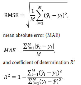
Here, yi is the observed target value,  is the average target value, and ŷi is the inferred (predicted) target value. These metrics give an overall summary of how good the model inference is. However, there are some details that they cannot capture. For example, although they can tell whether model predictions are of 'good' or 'bad' quality, they cannot tell if the model can be improved (using current data).
Mutual information (MI) is a useful tool to assess the information content of predictors with respect to the response. MI between two random variables X and Y, I[X,Y], is defined as follows:
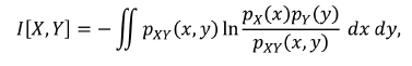
where integration is performed over the ange of values of X and Y and pX, pY, and pXY are probability density functions of X, Y, and their joint distribution respectively (Paninski, 2003). If variables X and Y are independent, it follows that I[X,Y] 0, since pXY = pX pY and the logarithm argument becomes unity. MI reaches a maximum when there is a purely functional relationship between the variables: by observing X one can precisely deduce Y. MI can be used to preselect the predictors or examine how important is the contribution of an individual predictor.
To facilitate the comparison between MI that corresponds to different predictors, it is useful to rescale MI and introduce relative MI, RMI, as follows (Cherkaev et al., 2022):
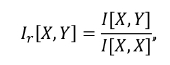
which ranges from 0 to 1 (or 0% to 100%). Thus, if RMIs between the response and all the predictors are low, it is not expected of any model to provide a useful inference of the response ('garbage in- garbage out').
Study objectives
This study aims to predict Si content in the tapped FeCr alloy using the data available up to the point when the tap starts. The methodology is similar to that of (Jonsson and Ingason (1998), but it extends the approach in the following ways:
► Si content is predicted per tap, not per day
► A wide range of predictors is used. Regularization methods are used to identify important predictors
► A nonlinear model is used to improve linear model results
► Variable importance is assessed.
The rest of the paper is structured as follows. An overview of the data used for the study is followed by a description of the steps taken for data preparation (steps 1-4 of the ML model framework). Dimensionality reduction and regression model development are sthen shown, followed by an assessment of the model performance and variable importance. Analysis of residuals assesses the possibility of improving the model. Finally, a general discussion and conclusions are presented.
Process monitoring data in FeCr smelting
Furnace process monitoring data comprises three distinct aspects: regular process monitoring data (named here tag data), tap data, and recipe and KPI (key performance indicator) data.
The outputs of temperature and electrical signal sensors are recorded at high frequency to tag data. Here 'high frequency' means that data is recorded most often. In many operations such data is recorded manually on an hourly basis. In this study, tag data was recorded automatically and sampled every 2 minutes. The recorded data includes hearth and shell temperatures, electrode currents, electrode holder positions, and power attributed to each electrode. Due to malfunction of some of the sensors, the data-set contains a considerable number of missing entries. Overall, it contains 130 variables and 2 412 000 observations.
The results of the analysis of the chemical compositions of tapped slag and alloy are recorded in tap data. Tap data is considered 'medium frequency' in this study as it is recorded on average every 3.2 hours. Since the analysis requires some time to perform, this data is not recorded online. The tap data contains 70 variables and 11 648 observations.
Recipeand KPI data (recipes data for short) is recorded daily and summarizes, among other indicators, the amounts and sources of different raw materials (reductant, flux, and ore) used. Since there are many sources and categories of, for example, reductant, recipe data is sparse: 57% of all entries are zero. The recipe data-set contains 156 variables and 1556 observations.
Data-set preparation
Embedding
Given the long processing times of a typical SAF, it is expected that not only most recently observed feature values, but also past values of features and the target, will influence future target value. To account for this influence, time embedding (see ML model framework subsection for more details) on the data-set was performed. It requires choosing the time shift step (delay interval) h and dimensionality k of the embedding. Although there are statistical methods to determine these parameters, they rely heavily on stationarity of the time series. Technical data in the processing industry is rarely stationary in the statistical sense, and these methods often fail. A more reliable way to determine these parameters is to use domain-specific knowledge. For example, it cannot be expected to see the effects of recipe changes past two days. As for the tap data, a study on ferromanganese smelting (Cherkaev et al., 2022) showed that it is not necessary to choose the dimensionality k > 2.
Tag data is not embedded in this study since tag data represents immediate furnace conditions that have only a short-term effect. Tap data is embedded with n = 2, i.e., two previous taps are considered with the current tap entry. Similarly, recipe data is embedded with dimensionality n = 2.
One notable consequence of embedding is the considerable increase in the number of variables. Both, tap data and recipe data increased the number of variables three times for n = 2.
Synchronization
Working with three separate data-sets is not convenient. Thus, the data-sets were combined to form a single set. Tap data was used as the base. Since there are many observations in tag data corresponding to a single entry in tap data, i.e., there are many observations from the previous tap start to the current tap start, these were replaced by a mean value. Furthermore, to account for tag data variability, an additional variable was introduced: the standard deviation of the original variable between the taps. To summarize, each tag variable X with values xn,xn+i , ... ,xn+k between the tap opening times is replaced by two variables:
each containing a single observation per tap. Recipe data was extended with zero-hold (last value carried forward) to provide one entry per tap.
Finally, current day recipe and current tap entries were excluded from the set of features since they cannot act as predictors for the current tap: they are available either at the end of the day or after the current tap is complete.
As a result of synchronization, dropping the variables that contain too many missing values and dropping the rows with missing tap data, the combined data-set contains 745 variables and 11 511 observations.
Training, testing, and validation data
The combined data-set was split into training, testing, and final validation sets. Thanks to time embedding performed on tap and recipe data, each entry in the data-set is independent of previous entries. Thus, training and testing samples can be drawn randomly from the data. For the final assessment of the model performance it is, however, more instructive to draw a continuous sample.
First, 200 contiguous observations were drawn from the middle of the data-set for the final validation data; 70% of the rest of the observations were randomly chosen for training, and the remainder were assigned for testing. This resulted in training and testing data having 8057 and 3254 observations respectively.
Standardization
The training data-set was used to calculate the mean and variance for each variable. These values were used to standardize all data-sets - training, testing, and validation.
Model development
This section presents the development of the data-driven model to predict Si content. All the development is done using the training data-set.
Dimensionality reduction
The high dimensionality of the data is a serious issue as it causes the variable-space to be only sparsely populated by observations. Furthermore, it is likely that the data contains many correlated variables. PCA was performed on the training set. Since PCA cannot process missing values directly, observations that contain them were removed from the data-set. The dimensionality reduction was performed by retaining the first 124 components that account for 90% of the total variance.
Linear model
Linear models have two attractive properties: they are cheap to train and easy to interpret. Thus, if there is a linear relationship between predictors and the response (Si content), it is advisable to extract it using a specialized linear model instead of relying on more general nonparametric models.
Similarly to PCA, linear models such as ordinary linear least squares (OLS), regularized OLS, or partial least squares (PLS) cannot handle missing values directly. The same approach as for PCA was followed: only the observations without missing values were used for training. LASSO linear regression was chosen as a linear model since it produces a sparse model (reduces the number of predictors), which helps model interpretation. The shrinkage parameter was automatically tuned during the learning procedure. The LASSO model was able to reduce the number of predictors from 124 to 84.
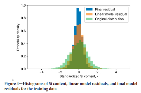
The LASSO model was able to reduce the variance of Si content on the training data-set from 1 (in standardized form) to 0.49. The distribution of residuals for the training data-set is shown in Figure 4. There is still a significant variability of residuals, which it is desirable to reduce. For this a nonlinear model needs to be employed.
Gradient boosting
It is assumed that the model is additive:
where residuals contain variability that was not explained by a linear model. These residuals are modelled using a gradient boosting (GB) method as implemented by the LightGBM package. GB involves a number of hyperparameters such as depth of individual trees, learning rate, and regularization parameters. A grid search was employed with 5-fold cross-validation to fine-tune these parameters. The final model was trained on the full training data-set with the fine-tuned hyperparameters.
Model performance
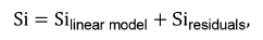
Model performance on training data
Although it is not possible to judge model performance when the model is applied to training data, it provides the base for comparison when applied to the testing data. Furthermore, it can give an idea of how effective model training was.
The coefficient of determination R2, MAE, and RMSE for both the linear model and the combined model are shown in Table I. Figure 4 compares the distributions of Si content, the linear model residuals, and the combined model residuals. It is evident that each model provides a considerable reduction in residuals variability. This is especially true for the addition of the GB model.
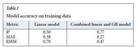
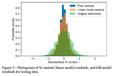
Model performance on testing data
Performance on the testing data is shown in Table II and Figure 5. The performance indicators of the linear model on the testing data are similar to those on the training data. In contrast, the combined model shows much less variability reduction compared to the training data. Nonetheless, there is still considerable reduction in variability by both linear and nonlinear models.
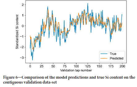
Validation on contiguous data
The result of the model applied to the contiguous data is shown in Figure 6. It is evident that although some variability in measured Si content is missed, model predictions provide an improved and reliable estimate compared to mean value (zero).
Importance of variables
For the purpose of Si content control, it is not enough to only predict it, but it is necessary to identify factors that affect it. While it is possible to point out several physical factors that control Si content, it is difficult to identify a particular factor that drives it up or down. Machine learning models provide a few techniques to identify the most important predictors of the model output. Linear models, including regularized models such as LASSO, offer a direct way for this by inspecting the model coefficients. GB models offer variable importance ranking as a part of the learning algorithm. However, for the current study this method is suboptimal since a GB model is used to improve the linear model results. A more direct approach for ranking variable importance is to use a permutation method, by which the observations of each variable are shuffled and the reduction in model accuracy is assessed.
Features selected by the LASSO linear regression model
Since the LASSO model was applied to the result of PCA transformation, they need to be considered together. PCA transformation can be represented as follows:
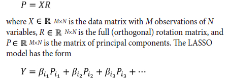
where Y is the response (Si content), Pj is the j-th column of P, ß} are non-zero coefficients of the LASSO model, and the ellipsis is used to show that other components were omitted. Combining this equation with PCA transformation gives:
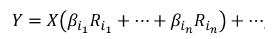
where Ri is the i-th column of matrix R. Since all the variables in matrix X have zero mean and variance unity (after standardization), their contribution can be assessed by the magnitude of the entries of the vector
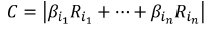
The first four largest entries of vector C correspond to Si content in the last two taps and average Si content in the last two days. This shows the strong autoregressive nature of the model. Other strong predictors include carbon and titanium content in metal in the previous tap, CaO content in the slag, and slag basicity.
Variables importance of the full model
The top importance predictors that were identified by the permutation importance method include past Si content values, carbon content in the previous tap (the second most important), electrode resistance, and electrode slip.
Analysis of residuals
Normality test
The Shapiro-Wilk normality test indicates that the combined model residuals are not Gaussian (p-value is 1.25x10⁻²⁵). Therefore, it is likely that there are a small number of factors that can further reduce their variability and, thus, improve the model.
Mutual information
Mutual information analysis was performed on the testing data-set to determine if there are predictors in the current data-set that can have a functional relationship with residuals. Predictors with more than 50% of missing values in the testing data-set were excluded from this analysis.
Compared to a fully deterministic model (i.e., residuals vs. residuals) taken as 100% MI, the largest MI between the residuals and predictors is 0.7%, corresponding to the active power standard deviation between the last and the current taps. For comparison, the top relative MI between the predictors and Si content is 7.5%. Low values of MI between the predictors for model residuals indicate that it is unlikely that the current model can be improved using the same predictors.
Discussion
Effect of recipe
One curious outcome of the features importance analysis is the absence of any recipe-related variables. The most likely explanation for this is that the recipe is correctly designed for the process. Indeed, recipe adjustments are made to control, among other parameters, Si content in the metal. Therefore, for the learning procedure, changes in the recipe appear to have no effect on Si content. The best way to pick up the recipe effect would be to randomly change the recipe, or at least to forgo Si content control in the recipe calculation. This, however, is impractical.
Selected features and thermodynamics
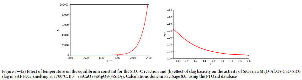
The features from the model, specifically the carbon and titanium contents of the alloy in the previous tap, the CaO content and basicity of the slag, and electrode parameters reflect what fundamentally drives many reduction reactions in pyrometallurgical processes, i.e. the relative effects of chemistry and temperature.
Consider the main reaction for SiO2 reduction in the furnace, repeated here for convenience:
The effect of temperature on the equilibrium constant for the reaction is given in Figure 7a. Although a simplistic view of a complex process, the temperature at which SiO2 reduction with carbon occurs has been shown to be almost overriding in SAF smelting of chromite (Haldar, 2020; Hayes, 2004) and largely due to improper heat input due to poor electrode control (James, Witten, Hastie, and Tibshirani, 2017) , i.e. if the resistance of the burden is such that the electrode tips sit high up in the furnace, a greater amount of energy is spent on a small volume of material, readily increasing the Si content of the alloy. Once Si is produced in a SAF process, the alloy droplets trickle to the bottom of the furnace. Very little can be done to refine the metal further, unlike, for example in open-bath chromite smelting processes (Hyvärinen, and Oja, 2000), where the alloy can still be refined by addition of highly basic oxides such as CaO.
This said, there is still a sound basis for the addition of basic oxides (e.g. CaO) to compensate for high Si contents of the alloy - if a mini-melt of high basicity slag forms close to the reaction sites for SiO2-C reaction, the activity of SiO2 in the melt can be suppressed to some degree by having a more basic slag, as shown in Figure 7b, limiting the extent to which the SiO2-C reaction is driven.
Reducible oxides in the slag, e.g. TiOx and VOx, naturally compete with CrOx and SiO2 in the slag for carbon. It is therefore not surprising that some of the minor elements in the alloy such as Ti come out as predictors for Si. Interaction between the alloy components can be described thermodynamically; however, the complexity and nonequilibrium nature of the SAF smelting process make it more difficult to do so. It is for this reason that a machine learning approach becomes invaluable. The effect of temperature (driven by electrical energy input from the electrodes) and chemistry effects are neatly combined into a practical model that can be used on the plant.
Conclusions
This study aimed to develop a data-driven Si content model and identify important drivers of Si content in FeCr smelting. The model, based on time-embedding, PCA, LASSO regression, and gradient boosting regression tree methods showed good predictive capabilities. The Si, C, and Ti contents in the metal and CaO content in the slag from the previous taps are among the strongest predictors of the Si content at he next tap. The importance of these predictors can be explained by the 'inertia' of a SAF (previous Si content) and chemical properties of the ore, reductant, and flux mixture. The absence of recipe-related variables as important features is probably due to the recipe being correctly designed. Analysis of residuals shows that it is unlikely that the current model can be improved any further (given the same data-set). Overall, this model can give an early warning sign to the operator if the Si content is moving away from the target.
Acknowledgements
The financial assistance of the National Research Foundation (NRF) toward this research is hereby acknowledged. Opinions expressed and conclusions arrived at are those of the author and are not necessarily to be attributed to the NRF.
This paper is published by permission of Mintek.
Conflict of interest
On behalf of all authors, the corresponding author states that there is no conflict of interest.
CRediT author statement
AVC: Methodology - Machine learning, Investigation, Formal analysis, Software, Writing, Visualisation, Project administration; ME: Methodology - Thermodynamics, Investigation, Writing, Visualisation; QGR: Supervision, Funding; SS: Conceptualisation, Supervision.
References
Boudraa, A-O. and Cexus, J-C. 2007. EMD-based signal filtering. IEEE Transactions on Instrumentation and Measurement, vol. 56. pp. 2196-2202. [ Links ]
Chatfield, C. 1996. The Analysis of Time Series. An Introduction. 5th edn. Chapman & Hall/CRC. [ Links ]
Cherkaev, A.V., Rampyapedi, K., Reynolds, Q.G., and Steenkamp, J.D. 2022. Tapped alloy mass prediction using data-driven models with an application to silicomanganese production. Furnace Tapping 2022. Springer. pp. 131-144. [ Links ]
Erwee, M., Swanepoel, S., and Reynolds, Q. 2021. The importance of controlling the chemistry of pre-oxidized chromite pellets for submerged arc furnace FeCr smelting: a study on furnace Si control. Proceedings of the 16th International Ferro-Alloys Congress (INFACON XVI) ,Trondheim, Norway, 27-29 September 2021. http://dx.doi.org/10.2139/ssrn.3926683 [ Links ]
Gasik, M.M. 2013. Introduction. Handbook of Ferroalloys. Elsevier. pp. 3-7. [ Links ]
Geldenhuys, I.J. 2013. Aspects of DC chromite smelting at Mintek - An overview. Proceedings of the Thirteenth International Ferroalloys Congress, Almaty, Kazakhstan, 9-13 June 2013. https://www.pyrometallurgy.co.za/InfaconXIII/0031-Geldenhuys.pdf [ Links ]
Haldar, S.K. 2020. Minerals and rocks. Introduction to Mineralogy and Petrology. Elsevier. pp. 1-51. [ Links ]
Hayes, P.C. 2004. Aspects of SAF smelting of ferrochrome. INFACON X: 'Transformation through Technology'. Proceedings of the Tenth International Ferroalloys Congress, Cape Town, South Africa, 1-4 February 2004. https://www.pyrometallurgy.co.za/InfaconX/046.pdf [ Links ]
Hockaday, S.A.C. and Bisaka, K. 2010. Some aspects of the production of ferrochrome alloys in pilot DC arc furnaces at Mintek. INFACON XII. Proceedingas of the 12th International Ferroalloys Congress, Helsinki, Finland. Outotek Oyj. pp. 367-376. [ Links ]
Hyvärinen, A. and Ota, E. 2000. Independent component analysis: algorithms and applications. Neural Networks, vol. 13. pp. 411-430. [ Links ]
James, G., Witten, D., Hastie, T., and Tibshirani, R. 2017. An Introduction to Statistical Learning with Applications in R. Springer. [ Links ]
Jonsson, G.R. and Lngason, H.T. 1998. On the control of silicon content in ferrosilicon. INFACON VIII. Proceedings of the 8th International Ferroalloys Congress, Beijing, China, 7-10 June 1998. China Science & Technology Press. pp. 95-98. [ Links ]
Luo, S. and Chen, T. 2020. Two derivative algorithms of gradient boosting decision tree for silicon content in blast furnace system prediction. IEEE Access, vol. 8. pp. 196112-196122. [ Links ]
Makridakis, S., Spiliotis, E., Assimakopoulos, v., Chen, Z., Gaba, A., Tsetlin, I., and Winkler, R.L. 2022. The M5 uncertainty competition: results, findings and conclusions. International Journal of Forecasting, vol. 38, no. 4. pp. 1365-1385. [ Links ]
Marwan, N., Romano, M.C., Thiel, M., and Kurths, J. 2007. Recurrence plots for the analysis of complex systems. Physics Reports, vol. 438. pp. 237-329. [ Links ]
McCoy, J.T. and Auret, L. 2019. Machine learning applications in minerals processing: a review. Minerals Engineering, vol. 132. pp. 95-109. [ Links ]
Paninski, L. 2003. Estimation of entropy and mutual information. Neural Computation, vol. 15. pp. 1191-1253. [ Links ]
Ranganathan, S. and Godiwalla, K.M. 2011. Influence of process parameters on reduction contours during production of ferrochromium in submerged arc furnace. Canadian Metallurgical Quarterly, vol. 50. pp. 37-44. [ Links ]
Ranganathan, S., Mishra, S.N., Mishra, R., and Singh, B.K. 2005. Control of silicon in high carbon ferrochromium produced in submerged arc furnace through redistribution of quartzite in the charge bed. Ironmaking & Steelmaking, vol. 32. pp. 177-184. [ Links ]
Ringdalen, E. and Eilertsen, J. 2001. Excavation of a 54 MVA HC-ferrochromium furnace. INFACON IX. Proceedings of the Ninth International Ferroalloys Congress. Quebec City, Canada, 3-6 June 2001. The Ferroalloys Association, Washinhton, DC. pp. 166-173. https://www.pyrometallurgy.co.za/InfaconIX/166-Ringdalen.pdf [ Links ]
Ringdalen, E., Rocha, M., and Figueiredo, P. 2015. Energy consumption during HCFeCr-production at Ferbasa. INFACON XIV. Proceedings of the Fourteenth International Ferroalloys Congress, Kiev, Ukraine, 31 May-4 June 2015. pp. 668-675. https://www.pyrometallurgy.co.za/InfaconXIV/668-Ringdalen.pdf [ Links ]
Urquhart, R. 1972. The production of high-carbon ferrochromium in a submerged-arc furnace. Minerals Science and Engineering, vol. 4. pp. 48-65. [ Links ]
Wedepohl, A. and Barcza, N.A. 1983. The 'dig-out' of a ferrochromium furnace. Special Publication no, 7. Geological Society of South Africa, Johannesburg. [ Links ]
Xiao, Y., Yang, Y., and Holappa, L. Tracking chromium behaviour in submerged arc furnace for ferrochrome production. Proeceedings of the Sohn International Symposium. Volume 7- Industrial Practice. Kongoli, F. and Reddy, R.G. (eds). TMS, Warrendale, PA. pp. 417-433. [ Links ]
 Correspondence:
A.V. Cherkaev
Email:Alexey.Cherkaev@SamancorCr.com
Received: 31 Aug. 2022
Revised: 11 Dec. 2022
Accepted: 13 Dec. 2023
Published: February 2024

